Meta-analysis of movement-model parameters

These functions estimate population-level mean parameters from individual movement models and related estimates, including AKDE home-range areas, while taking into account estimation uncertainty.

meta(x,variable="area",level=0.95,level.UD=0.95,method="MLE",IC="AICc",boot=FALSE,
     error=0.01,debias=TRUE,verbose=FALSE,units=TRUE,plot=TRUE,sort=FALSE,mean=TRUE,
     col="black",...)

funnel(x,y,variable="area",precision="t",level=0.95,level.UD=0.95,...)

Arguments

x

A named list of ctmm movement-model objects, UD objects, UD summary output, speed output, or 2\(\times\)2 overlap objects constituting a sampled population, or a named list of such lists, with each constituting a sampled population.

y

An optional named list of telemetry objects for the funnel-plot precision variable.

variable

Biological ``effect'' variable of interest for ctmm object arguments. Can be "area", "diffusion", "speed", "tau position", or "tau velocity".

precision

Precision variable of interest. Can be "t" for sampling time period or time interval, "n" for nominal sample size, "N" or "DOF" for effective sample size.

level

Confidence level for parameter estimates.

level.UD

Coverage level for home-range estimates. E.g., 50% core home range.

method

Statistical estimator used---either maximum likelihood estimation based ("MLE") or approximate `best linear unbiased estimator' ("BLUE")---for comparison purposes.

IC

Information criterion to determine whether or not population variation can be estimated. Can be "AICc", AIC, or "BIC".

boot

Perform a parametric bootstrap for confidence intervals and first-order bias correction if debias=TRUE.

error

Relative error tolerance for parametric bootstrap.

debias

Apply Bessel's inverse-Gaussian correction and various other bias corrections if method="MLE", REML if method="BLUE", and an additional first-order correction if boot=TRUE.

verbose

Return a list of both population and meta-population analyses if TRUE and x is a list of population lists.

units

Convert result to natural units.

plot

Generate a meta-analysis forest plot.

sort

Sort individuals by their point estimates in forest plot.

mean

Include population mean estimate in forest plot.

col

Color(s) for individual labels and error bars.

...

Further arguments passed to plot or meta.

Details

meta employs a custom \(\chi^2\)-IG hierarchical model to calculate debiased population mean estimates of positive scale parameters, including home-range areas, diffusion rates, mean speeds, and autocorrelation timescales. Model selection is performed between the \(\chi^2\)-IG population model (with population mean and variance) and the Dirac-\(\delta\) population model (population mean only). Population ``coefficient of variation'' (CoV) estimates are also provided. Further details are given in Fleming et al (2022).

Value

If x constitutes a sampled population, then meta returns a table with rows corresponding to the population mean and coefficient of variation.

If x constitutes a list of sampled populations, then meta returns confidence intervals on the population mean variable ratios.

References

C. H. Fleming, I. Deznabi, S. Alavi, M. C. Crofoot, B. T. Hirsch, E. P. Medici, M. J. Noonan, R. Kays, W. F. Fagan, D. Sheldon, J. M. Calabrese, ``Population-level inference for home-range areas'', Methods in Ecology and Evolution 13:5 1027--1041 (2022) doi:10.1111/2041-210X.13815 .

Author

C. H. Fleming.

Note

The AICc formula is approximated via the Gaussian relation.

Confidence intervals depicted in the forest plot are \(\chi^2\) and may differ from the output of summary() in the case of mean speed and timescale parameters with small effective sample sizes.

As mean ratio estimates are debiased, reciprocal estimates can differ slightly.

See also

akde, cluster, ctmm.fit.

Examples

# \donttest{
# load package and data
library(ctmm)
data(buffalo)

# fit movement models
FITS <- AKDES <- list()
for(i in 1:length(buffalo))
{
  GUESS <- ctmm.guess(buffalo[[i]],interactive=FALSE)
  # use ctmm.select unless you are certain that the selected model is OUF
  FITS[[i]] <- ctmm.fit(buffalo[[i]],GUESS)
}

# calculate AKDES on a consistent grid
AKDES <- akde(buffalo,FITS)
#> Default grid size of 3 minutes chosen for bandwidth(...,fast=TRUE).
#> Default grid size of 2 minutes chosen for bandwidth(...,fast=TRUE).
#> Default grid size of 2 minutes chosen for bandwidth(...,fast=TRUE).
#> Default grid size of 3 minutes chosen for bandwidth(...,fast=TRUE).
#> Default grid size of 2 minutes chosen for bandwidth(...,fast=TRUE).
#> Default grid size of 5 minutes chosen for bandwidth(...,fast=TRUE).

# color to be spatially distinct
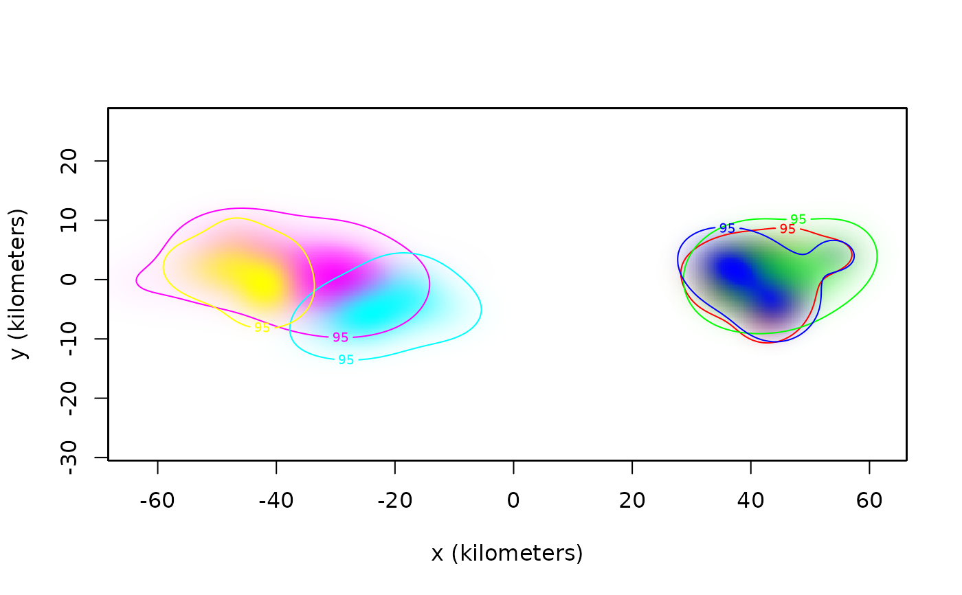
COL <- color(AKDES,by='individual')

# plot AKDEs
plot(AKDES,col.DF=COL,col.level=COL,col.grid=NA,level=NA)


# meta-analysis of buffalo home-range areas
meta(AKDES,col=c(COL,'black'),sort=TRUE)
#>                    ΔAICc
#> Dirac-δ          0.00000
#> inverse-Gaussian 3.83404

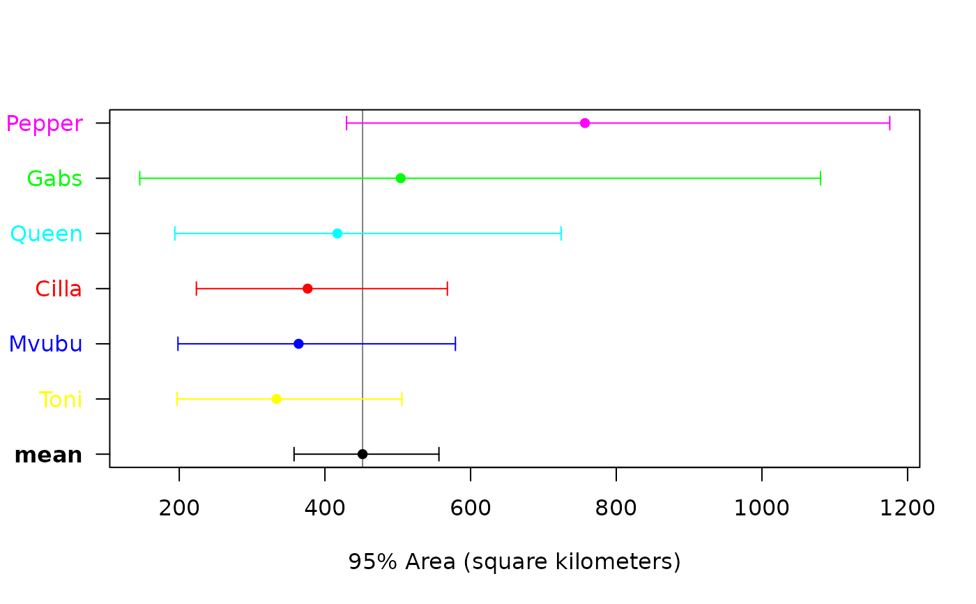#>                low      est     high
#> mean (km²)  357.63 451.6816 556.5468
#> CoV² (RVAR)   0.00   0.0000      Inf
#> CoV  (RSTD)   0.00   0.0000      Inf

# funnel plot to check for sampling bias
funnel(AKDES,buffalo)

# }