Clustering of movement-model parameters

These functions cluster and classify individual movement models and related estimates, including AKDE home-range areas, while taking into account estimation uncertainty.

cluster(x,level=0.95,level.UD=0.95,debias=TRUE,IC="BIC",units=TRUE,plot=TRUE,sort=FALSE,
        ...)

Arguments

x: A list of ctmm movement-model objects, UD objects, or UD summary output, constituting a sampled population, or a list of such lists, each constituting a sampled sub-population.
level: Confidence level for parameter estimates.
level.UD: Coverage level for home-range estimates. E.g., 50% core home range.
debias: Apply Bessel's inverse-Gaussian correction and various other bias corrections.
IC: Information criterion to determine whether or not population variation can be estimated. Can be "AICc", AIC, or "BIC".
units: Convert result to natural units.
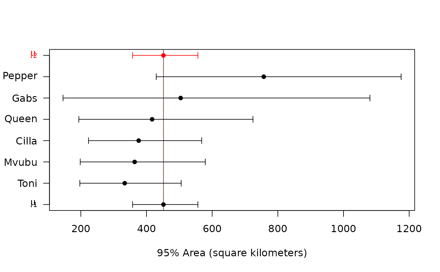
plot: Generate a meta-analysis forest plot with two means.
sort: Sort individuals by their point estimates in forest plot.
...: Further arguments passed to plot.

Details

So-far only the clustering of home-range areas is implemented. More details will be provided in an upcomming manuscript.

Value

A list with elements P and CI, where P is an array of individual membership probabilities for sub-population 1, and CI is a table with rows corresponding to the sub-population means, coefficients of variation, and membership probabilities, and the ratio of sub-population means.

Author

C. H. Fleming.

Note

The AICc formula is approximated via the Gaussian relation.

Examples

# \donttest{
# load package and data
library(ctmm)
data(buffalo)

# fit movement models
FITS <- AKDES <- list()
for(i in 1:length(buffalo))
{
  GUESS <- ctmm.guess(buffalo[[i]],interactive=FALSE)
  # use ctmm.select unless you are certain that the selected model is OUF
  FITS[[i]] <- ctmm.fit(buffalo[[i]],GUESS)
}

# calculate AKDES on a consistent grid
AKDES <- akde(buffalo,FITS)
#> Default grid size of 3 minutes chosen for bandwidth(...,fast=TRUE).
#> Default grid size of 2 minutes chosen for bandwidth(...,fast=TRUE).
#> Default grid size of 2 minutes chosen for bandwidth(...,fast=TRUE).
#> Default grid size of 3 minutes chosen for bandwidth(...,fast=TRUE).
#> Default grid size of 2 minutes chosen for bandwidth(...,fast=TRUE).
#> Default grid size of 5 minutes chosen for bandwidth(...,fast=TRUE).

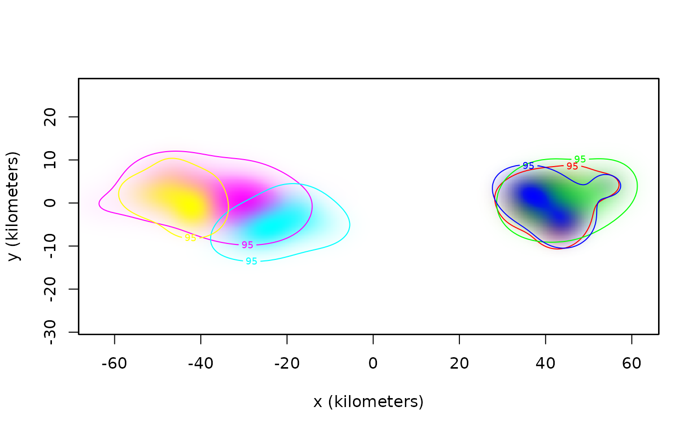
# color to be spatially distinct
COL <- color(AKDES,by='individual')

# plot AKDEs
plot(AKDES,col.DF=COL,col.level=COL,col.grid=NA,level=NA)


# cluster-analysis of buffalo
cluster(AKDES,sort=TRUE)
#>                                                      ΔBIC
#> Dirac-δ                                         0.0000000
#> inverse-Gaussian                                0.9591028
#> Dirac-δ + Dirac-δ                               1.3582120
#> inverse-Gaussian(CoV) + inverse-Gaussian(CoV)   3.1499715
#> Dirac-δ + inverse-Gaussian                      3.1499715
#> inverse-Gaussian + Dirac-δ                      3.1499715
#> inverse-Gaussian(CoV₁) + inverse-Gaussian(CoV₂) 4.9417310

#> $P
#>  Cilla   Gabs  Mvubu Pepper  Queen   Toni 
#>      1      1      1      1      1      1 
#> 
#> $CI
#>              low      est     high
#> μ₁ (km²) 357.629 451.6807 556.5461
#> CoV₁       0.000   0.0000      Inf
#> μ₂ (km²) 357.629 451.6807 556.5461
#> CoV₂       0.000   0.0000      Inf
#> P₁         0.000   1.0000   1.0000
#> P₂         0.000   0.0000   1.0000
#> μ₂/μ₁      0.000   1.0000      Inf
#> 
# }