Error calibration
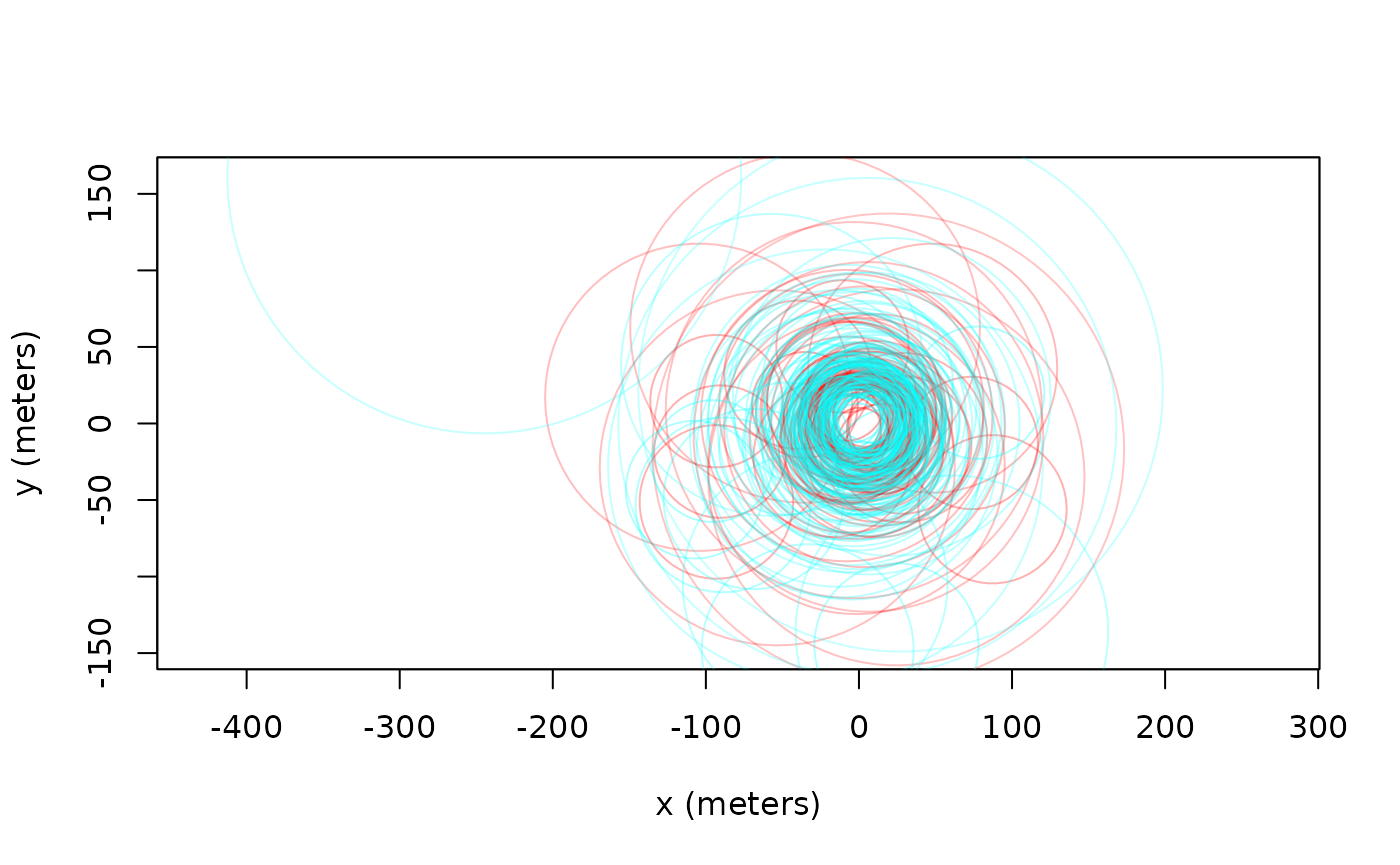
The first step to handling errors is to quantify them. Make sure that your data’s “dilution of precision” (DOP) and error columns import correctly into ctmm. In the following wood turtle dataset, we have some calibration data and a turtle track. Note that the calibration data must be collected from the same model device as the tracking data, and their data formatting bust be similar enough that the same location classes are detected by as.telemetry.
## The legacy packages maptools, rgdal, and rgeos, underpinning the sp package,
## which was just loaded, will retire in October 2023.
## Please refer to R-spatial evolution reports for details, especially
## https://r-spatial.org/r/2023/05/15/evolution4.html.
## It may be desirable to make the sf package available;
## package maintainers should consider adding sf to Suggests:.
## The sp package is now running under evolution status 2
##      (status 2 uses the sf package in place of rgdal)
data(turtle)
names(turtle[[1]]) # data are not yet calibrated, but HDOP and location class is present
## [1] "t" "HDOP" "class" "x" "y"
names(turtle) # two calibration datasets and two turtle datasets## [1] "60s" "90s" "F231" "F403"
The uere command is used to estimate the RMS UERE parameter(s) from calibration data. Do not use this command on animal tracking data.
## , , horizontal
##
##          low       est      high
## 2D 22.786528 29.598802 36.397467
## 3D  6.477391  6.946024  7.414237
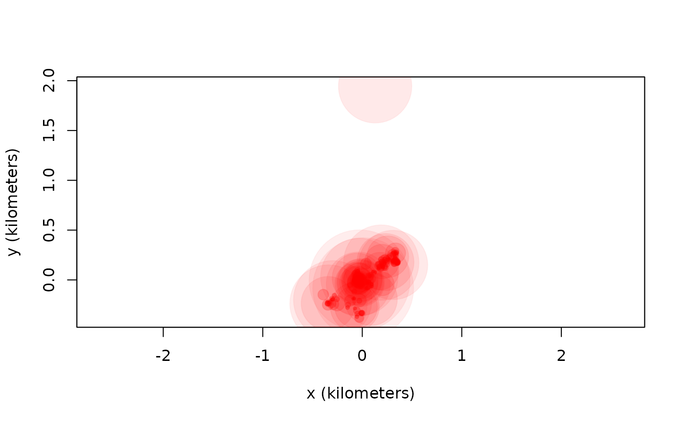
For GPS data, the RMS UERE will typically be 10-15 meters. Here we have two location classes, “2D” and “3D”, which for this device have substantially different RMS UERE values. The UERE parameters can then be assigned to a dataset with the uere()<- command.
## , , horizontal
##
##          low       est      high
## 2D 22.786528 29.598802 36.397467
## 3D  6.477391  6.946024  7.414237
plot(turtle[[3]],error=2) # turtle plot with 95% error discs
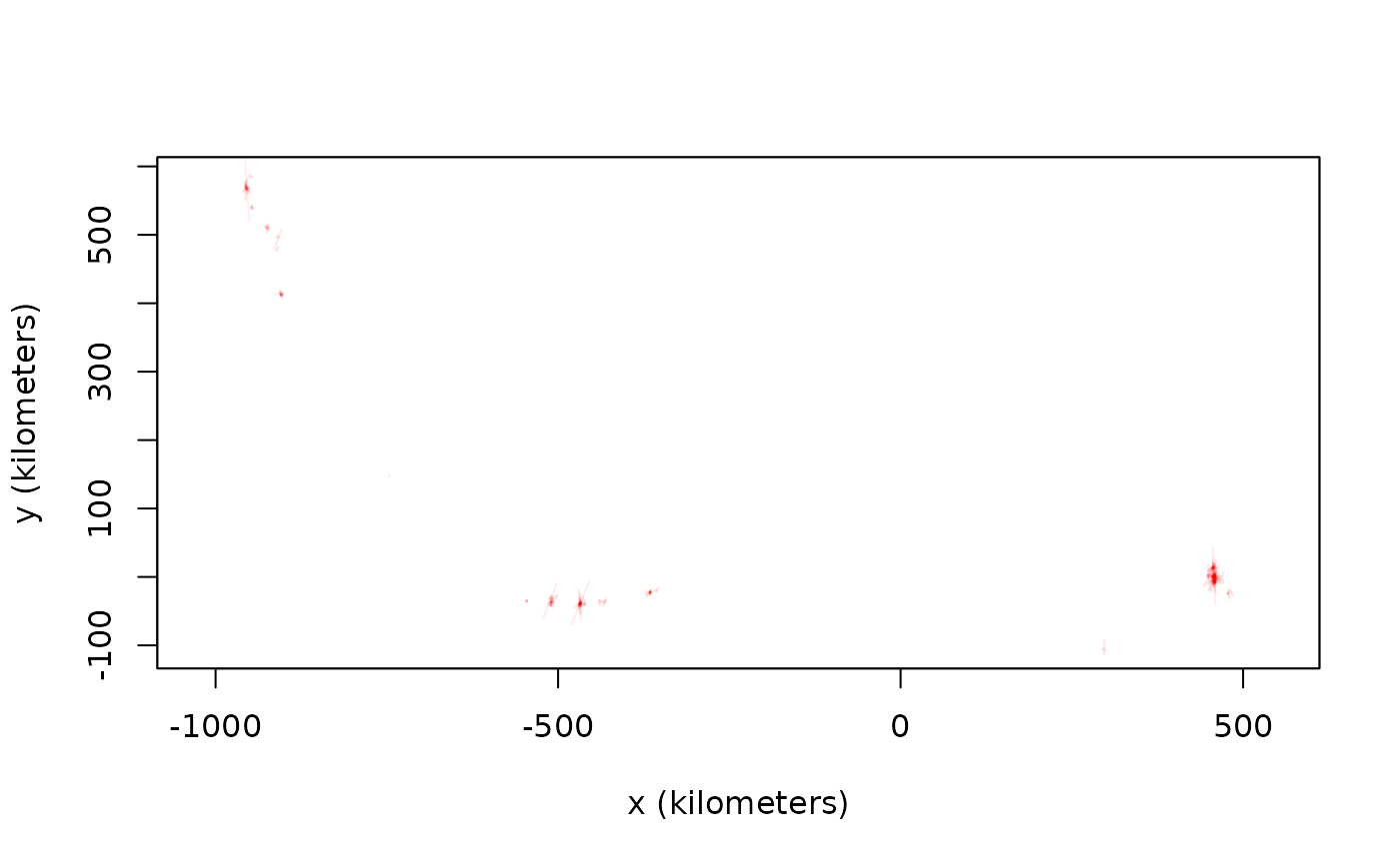
If you have Argos data, they will import with calibration already applied to the horizontal dimensions, but not the vertical dimension.
## [1] "gps" "argos"
names(pelican$argos) # error ellipse information (COV and VAR) already present## [1] "timestamp" "longitude" "latitude" "t" "COV.angle" "HDOP"
## [7] "COV.major" "COV.minor" "VAR.xy" "class" "z" "VDOP"
## [13] "x" "y" "COV.x.x" "COV.x.y" "COV.y.y"
plot(pelican$argos) # pelican Argos plot with 95% error ellipses
Error model selection
Not all GPS devices provide reliable DOP values and sometimes it is not obvious what error information will prove to be the most predictive. Generally speaking, as.telemetry will attempt to import the “best” column from among those that estimate error, DOP value, number of satellites and fix type, including timed-out fixes (see the timeout argument in help(as.telemetry)). Researchers may want to import their data with different error information, run uere.fit for each error model, and then select among the candidate models. Here we do this by comparing the turtle calibration data with and without HDOP values.
First, we consider whether or not the HDOP and location class information are informative.
t.noHDOP  <- lapply(turtle,function(t){ t$HDOP  <- NULL; t })
t.noclass <- lapply(turtle,function(t){ t$class <- NULL; t })
t.nothing <- lapply(turtle,function(t){ t$HDOP  <- NULL; t$class <- NULL; t })
In other cases, manipulation will need to be performed before importing, so that as.telemetry can format the telemetry object properly. Running uere.fit now results in errors calibrated under the assumption of homoskedastic errors.
UERE.noHDOP  <- uere.fit(t.noHDOP[1:2])
UERE.noclass <- uere.fit(t.noclass[1:2])
UERE.nothing <- uere.fit(t.nothing[1:2])
We can now apply model selection to the UERE model fits by summarizing them in a list.
##                  ΔAICc  Z[red]²
## HDOP.class      0.0000 2.366617
## HDOP          286.5747 3.908826
## class         418.5174 3.696585
## homoskedastic 637.2580 4.681067
We can see that the combination of location class and HDOP values yield the best error model, both in terms of AICc and in terms of reduced Z squared. Reduced Z squared is a goodness-of-fit statistic akin to reduced chi squared, but designed for comparing error models.
We had two calibration datasets, so we can also see if there is any substantial difference between the two GPS tags. We do this by making a list of individual UERE objects to compare to the previous joint UERE model.
##               ΔAICc  Z[red]²
## joint      0.000000 2.366617
## individual 3.314758 2.367412
In this case, performance of the individualized and joint error models are comparable, and AICc selects the joint model.
Outlier detection
Now we come to the task of identifying outliers. The outlie function uses error information to estimate straight-line speeds between sampled times and distances from the bulk of the data.
outlie(turtle[[3]]) -> OUT
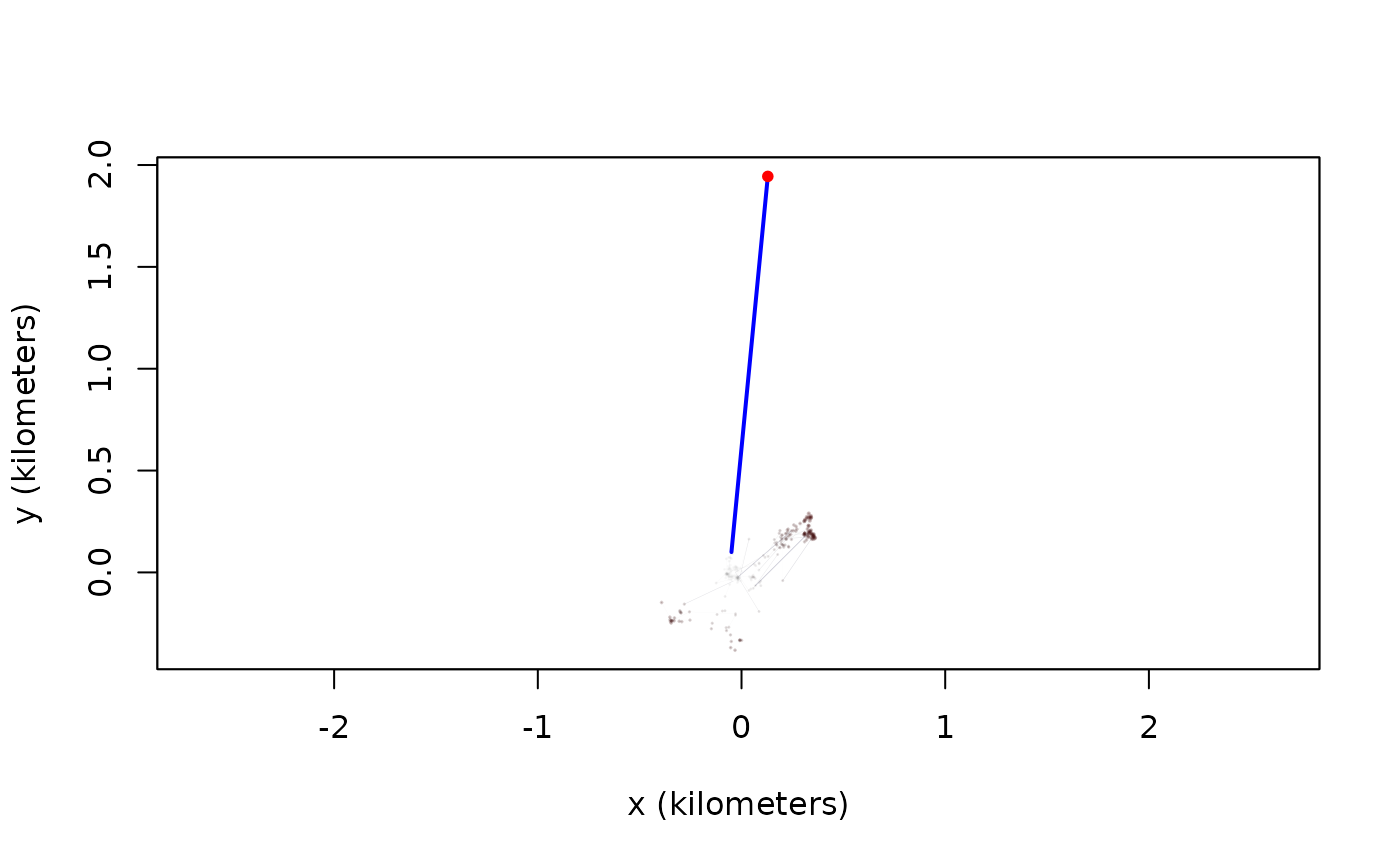
High-speed segments are colored in blue, while distant locations are colored in red. More emphasis is placed on the more extreme locations in the outlie plot. Visually we can see at least one outlier in the wood turtle data. The output of outlie also contains the error-informed speed and distance estimates (in SI units) used to generate the plot.
plot(OUT,units=FALSE)
A sustained speed of 0.1 m/s is not biologically implausible for a wood turtle, but this location is highly suspicious, both in terms of speed and lack of proximity. After removing the outlier, we can check the data again.
BAD <- OUT$speed>0.08 # not appropriate for other species!
turtle[[3]] <- turtle[[3]][!BAD,]
outlie(turtle[[3]]) -> OUT
Datasets may have multiple outliers. In pathological situations, there may be no clear separation between the normative data and the outliers. This necessitates a better error model, either by improving inadequate (or absent) HDOP estimates or by employing a heavier tailed error distribution (not yet supported).
Variograms and model selection
Variograms
If we were working with Argos data or high resolution GPS data on a small animal, then we can get a “nugget” effect in the variogram that looks like an initial discontinuity at short time lags.


The height of this initial discontinuity corresponds to the variance of uncorrelated location errors. The second plot is the kind of initial discontinuity one has with detector array data. The end of the (slope) discontinuity is highlighted with a circle. This discontinuity is smooth because the movement and detection are correlated. The height of this initial discontinuity is also (at least roughly) the variance of the location errors.
Model fitting
Because of some convenient mathematical relations, fitting with telemetry errors involves numerically fitting 1-4 more parameters and is, therefore, slower and less reliable at converging on the MLE than fitting without telemetry error. Therefore, by default, telemetry error is not turned on in ctmm models (error=FALSE). Furthermore, in cases with an error model, ctmm.select() is safer to use than direct applicaiton of ctmm.fit(), because ctmm.select() will start with the simplest “compatible” model and then consider further model features that require numerical optimization in stepwise fashion.
Fitting with calibrated data
For calibrated errors, we have to set error=TRUE in the model guess to fit with telemetry error accounted for.
# automated guesstimate for calibrated data
GUESS <- ctmm.guess(turtle[[3]],CTMM=ctmm(error=TRUE),interactive=FALSE)
# stepwise fitting # CRAN policy limits us to 2 cores
FIT <- ctmm.select(turtle[[3]],GUESS,trace=TRUE,cores=2)
## * Fitting model OUF error## * Fitting model OUF anisotropic error## * Fitting model IID anisotropic error
# if you get errors on your platform, then try cores=1
summary(FIT)
## $name
## [1] "OU anisotropic error"
##
## $DOF
## mean area diffusion speed
## 13.90252 23.94155 194.84072 0.00000
##
## $CI
## low est high
## area (hectares) 13.619544 21.269510 30.597234
## τ[position] (days) 3.561604 5.684240 9.071918
## diffusion (square meters/day) 4663.853685 5394.799125 6178.175193
## error 2D (meters) 18.539407 21.885545 25.225778
## error 3D (meters) 6.590236 7.063699 7.536738trace=TRUE allows us to see the models considered. verbose=TRUE would save each model. Since we started with a finite amount of calibration data, the location-error parameter estimates were updated by the tracking data, and we can compare the results here with the previous estimates in summary(UERE).
Simultaneous fitting with uncalibrated data
Fitting with unknown errors is a method of last resort. We have to provide an initial guess for error, which will be the device’s RMS UERE. error=10 is usually a good guess for GPS data (other than e-obs). Unlike uere.fit, ctmm.fit is not yet coded to use the location classes, as simultaneous fitting is a method of last resort that becomes increasingly dangerous with more location classes.
# delete UERE information
uere(turtle) <- NULL
The only difference is that you have to provide an initial guess for the RMS UERE. Otherwise, the steps are the same.
# automated guesstimate for uncalibrated data (with 10 meter RMS UERE guess)
GUESS <- ctmm.guess(turtle[[3]],CTMM=ctmm(error=10),interactive=FALSE)
# fit and select models # CRAN policy limits us to 2 cores
FIT <- ctmm.select(turtle[[3]],GUESS,trace=TRUE,cores=2)
## * Fitting model OUF error## * Fitting model OUF anisotropic error## * Fitting model IID anisotropic error
# if you get errors on your platform, then try cores=1
summary(FIT)
## $name
## [1] "OU anisotropic error"
##
## $DOF
## mean area diffusion speed
## 12.85422 21.90112 140.47104 0.00000
##
## $CI
## low est high
## area (hectares) 13.034815 20.823830 30.40796
## τ[position] (days) 3.734213 6.186523 10.24930
## diffusion (square meters/day) 4229.458030 5026.254306 5890.79677
## error 2D (meters) 7.750780 10.815976 13.87601
## error 3D (meters) 6.940370 8.749010 10.55403Here, fitting the RMS UERE simultaneously with the movement model produced a largely consistent result. This will not always be the case.
Fitting with uncalibrated data under a prior
An alternative method of last resort is to simply assign a range of credible RMS UERE values to the data. Again, 10-meter error is usually a good guess for 3D GPS data. For e-obs, and other devices that report error in meters, a number on the order of 1 is usually more relevant.
## , , horizontal
##
##    low est high
## 2D   0   1  Inf
## 3D   0   1  Inf
# assign 20-meter 2D RMS UERE and 10-meter 3D RMS UERE
uere(turtle) <- c(20,10)
# for one location class, the above would likely be unnecessary, but would look like
# uere(turtle) <- 10

# the default uncertainty is none for numerical assignments
UERE <- uere(turtle)
summary(UERE)
## , , horizontal
##
## low est high
## 2D 20 20 20
## 3D 10 10 10
# this is because the degrees-of-freedom are set to Inf
UERE$DOF
## horizontal
## 2D Inf
## 3D Inf
# here I set the DOF to a smaller value
UERE$DOF[] <- 2
# which now gives plausible credible intervals
summary(UERE)
## , , horizontal
##
## low est high
## 2D 6.960018 20 33.38156
## 3D 3.480009 10 16.69078
# assign the prior to the data
uere(turtle) <- UERE
# automated guesstimate for calibrated data
GUESS <- ctmm.guess(turtle[[3]],CTMM=ctmm(error=TRUE),interactive=FALSE)
# stepwise fitting # CRAN policy limits us to 2 cores
FIT <- ctmm.select(turtle[[3]],GUESS,trace=TRUE,cores=2)
## * Fitting model OUF error## * Fitting model OUF anisotropic error## * Fitting model IID anisotropic error
# if you get weird errors on your platform, then try cores=1
summary(FIT)
## $name
## [1] "OU anisotropic error"
##
## $DOF
## mean area diffusion speed
## 12.70947 21.64740 143.50521 0.00000
##
## $CI
## low est high
## area (hectares) 12.966262 20.777867 30.40155
## τ[position] (days) 3.773826 6.262912 10.39371
## diffusion (square meters/day) 4197.634099 4978.897600 5825.85083
## error 2D (meters) 9.462815 12.388806 15.30899
## error 3D (meters) 7.186924 8.889062 10.58785This method is still being developed and so this material is subject to change.