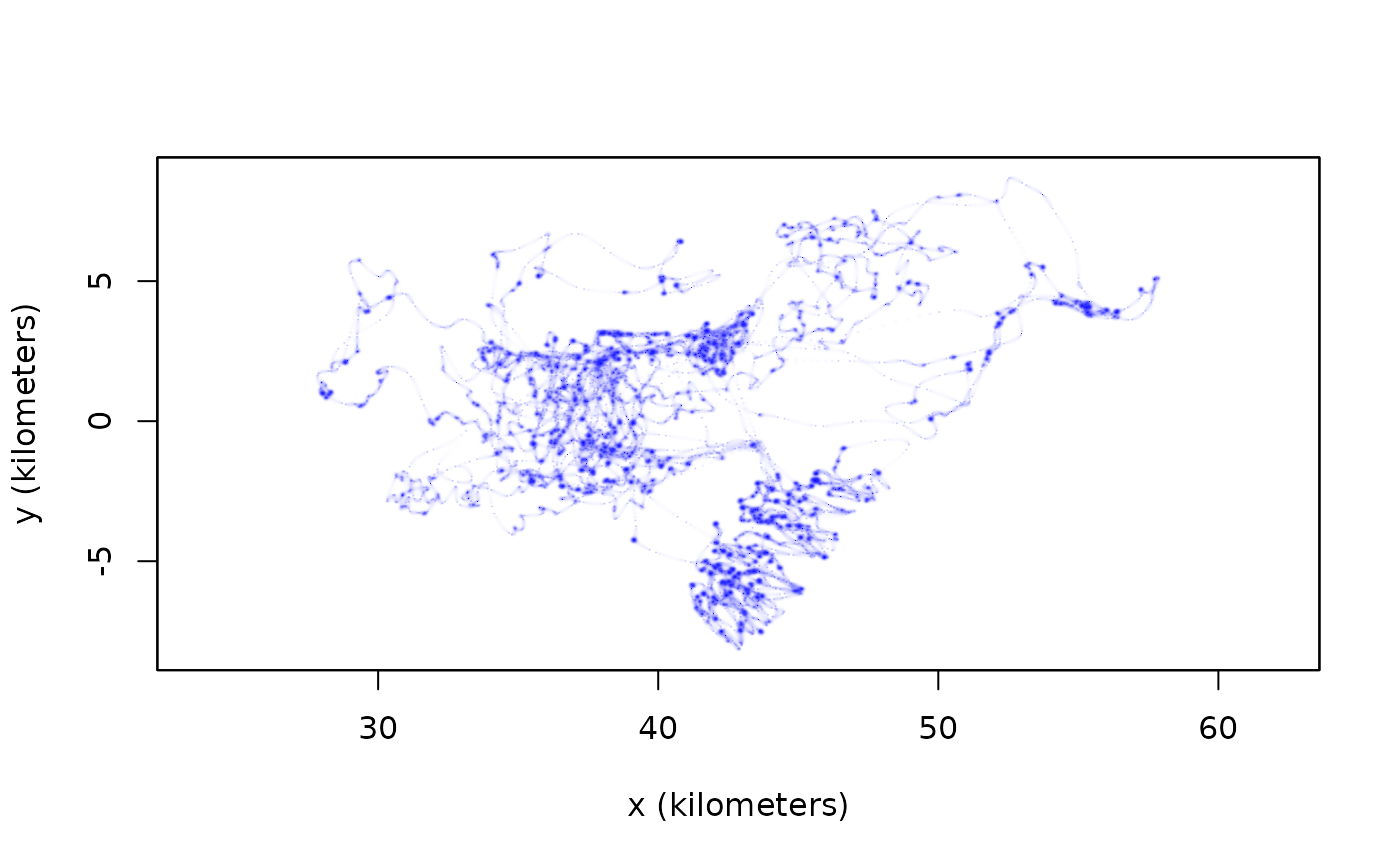
Calculate a Kriged occurrence distribution estimate

This function calculates an occurrence distribution from telemetry data and a continuous-time movement model.

occurrence(data,CTMM,R=list(),SP=NULL,SP.in=TRUE,H=0,variable="utilization",res.time=10,
           res.space=10,grid=NULL,cor.min=0.05,dt.max=NULL,buffer=TRUE,...)

Arguments

data: A telemetry object or list of telemetry objects.
CTMM: A ctmm movement model, as from the output of ctmm.select, or a list of ctmm objects.
R: A named list of raster covariates if CTMM contains an RSF model.
SP: SpatialPolygonsDataFrame object for enforcing hard boundaries.
SP.in: Locations are assumed to be inside the SP polygons if SP.in=TRUE and outside of SP if SP.in=FALSE.
H: Optional additional bandwidth matrix for future use.
variable: Either "utilization" or "revisitation". Only utilization is accurately estimated.
res.time: Number of temporal grid points per median timestep.
res.space: Number of grid points along each axis, relative to the average diffusion (per median timestep) from a stationary point.
grid: Optional grid specification via raster, UD, or list of arguments (See akde for details).
cor.min: Velocity correlation threshold for skipping gaps.
dt.max: Maximum absolute gap size (in seconds) for Kriging interpolation. If left NULL, the median of diff(data$t) will be used.
buffer: Buffer the observation period, according to the minimum gap specified by cor.min and dt.max, to include more probable locations if possible.
...: Not used.

Details

The arguments cor.min or dt.max are used to prevent the interpolation of large gaps, which would bias the estimate to more resemble the movement model than the data. Because cor.min can produce an empty range with fractal movement models, the larger of the two rules is employed for interpolation.

If buffer=TRUE, then the data are also extrapolated according to the minimum of the two rules (cor.min and dt.max) which is limited to cases where persistence of motion is modeled.

Value

Returns a UD object containing the sampled grid line locations x and y, the probability density and cumulative distribution functions evaluated on the sampled grid locations PDF & CDF, the optional bandwidth matrix H, and the area of each grid cell dA.

References

C. H. Fleming, W. F. Fagan, T. Mueller, K. A. Olson, P. Leimgruber, J. M. Calabrese, ``Estimating where and how animals travel: An optimal framework for path reconstruction from autocorrelated tracking data'', Ecology, 97:3, 576-582 (2016) doi:10.1890/15-1607.1 .

C. H. Fleming, D. Sheldon, E. Gurarie, W. F. Fagan, S. LaPoint, J. M. Calabrese, ``Kálmán filters for continuous-time movement models'', Ecological Informatics, 40, 8-21 (2017) doi:10.1016/j.ecoinf.2017.04.008 .

Author

C. H. Fleming.

Note

Large gaps have a tendency to slow down computation and blow up the estimate. This can be avoided with the cor.min or dt.max arguments.

In the case of coarse grids, the value of PDF in a grid cell actually corresponds to the average probability density over the entire rectangular cell.

Prior to ctmm v0.5.6, cor.min referred to the location correlation, with a default of 50%. In ctmm v0.5.6 and above, cor.min refers to the velocity correlation, with a default of 5%.

Examples

# \donttest{
# Load package and data
library(ctmm)
data(buffalo)
Cilla <- buffalo$Cilla

GUESS <- ctmm.guess(Cilla,interactive=FALSE)
FIT <- ctmm.fit(Cilla,GUESS)

# Compute occurence distribution
UD <- occurrence(Cilla,FIT)

# Plot occurrence UD
plot(UD,col.level=NA)

# }