Encounter statistics

Functions to calculate encounter probabilities and the conditional location distribution of where encounters take place (conditional on said encounters taking place), as described in Noonan et al (2021).

encounter(object,debias=FALSE,level=0.95,normalize=FALSE,self=TRUE,...)

cde(object,include=NULL,exclude=NULL,debias=FALSE,...)

Arguments

object: A list of aligned UD objects.
debias: Approximate bias corrections [IN DEVELOPMENT].
level: Confidence level for relative encounter rates.
normalize: Normalize relative encounter rates by the average uncorrelated self-encounter rate.
self: Fix the self-interaction rate appropriately.
include: A matrix of interactions to include in the calculation (see Details below).
exclude: A matrix of interactions to exclude in the calculation (see Details below).
...: Additional arguments for future use.

Details

Encounter probabilities are standardized to 1 meter, and must be multiplied by the square encounter radius (in meters), to obtain other values. If normalize=FALSE, the relative encounter rates have units of \(1/m^2\) and tend to be very small numbers for very large home-range areas. If normalize=TRUE, the relative encounter rates are normalized by the average uncorrelated self-encounter rate, which is an arbitrary value that provides a convenient scaling.

The include argument is a matrix that indicates which interactions are considered in the calculation. By default, include = 1 - diag(length(object)), which implies that all interactions are considered aside from self-interactions. Alternatively, exclude = 1 - include can be specified, and is by-default exclude = diag(length(object)), which implies that only self-encounters are excluded.

Value

encounter produces an array of standardized encounter probabilities with CIs, while cde produces a single UD object.

References

M. J. Noonan, R. Martinez-Garcia, G. H. Davis, M. C. Crofoot, R. Kays, B. T. Hirsch, D. Caillaud, E. Payne, A. Sih, D. L. Sinn, O. Spiegel, W. F. Fagan, C. H. Fleming, J. M. Calabrese, ``Estimating encounter location distributions from animal tracking data'', Methods in Ecology and Evolution (2021) doi:10.1111/2041-210X.13597 .

Author

C. H. Fleming

Note

Prior to v1.2.0, encounter() calculated the CDE and rates() calculated relative encounter probabilities.

Examples

# \donttest{
# Load package and data
library(ctmm)
data(buffalo)

# fit models for first two buffalo
GUESS <- lapply(buffalo[1:2], function(b) ctmm.guess(b,interactive=FALSE) )
# in general, you should use ctmm.select here
FITS <- lapply(1:2, function(i) ctmm.fit(buffalo[[i]],GUESS[[i]]) )
names(FITS) <- names(buffalo[1:2])

# create aligned UDs
UDS <- akde(buffalo[1:2],FITS)
#> Default grid size of 3 minutes chosen for bandwidth(...,fast=TRUE).
#> Default grid size of 2 minutes chosen for bandwidth(...,fast=TRUE).

# calculate 100-meter encounter probabilities
P <- encounter(UDS)
P$CI * 100^2
#> , , low
#> 
#>              Cilla         Gabs
#> Cilla          Inf 4.612574e-05
#> Gabs  4.612574e-05          Inf
#> 
#> , , est
#> 
#>             Cilla        Gabs
#> Cilla         Inf 9.17698e-05
#> Gabs  9.17698e-05         Inf
#> 
#> , , high
#> 
#>              Cilla         Gabs
#> Cilla          Inf 0.0001528501
#> Gabs  0.0001528501          Inf
#> 

# calculate CDE
CDE <- cde(UDS)

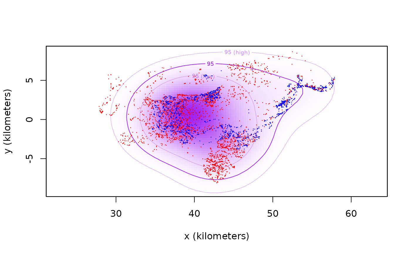
# plot data and encounter distribution
plot(buffalo[1:2],col=c('red','blue'),UD=CDE,col.DF='purple',col.level='purple',col.grid=NA)
#> DOP values missing. Assuming DOP=1.
#> DOP values missing. Assuming DOP=1.

# }