Introduction
This document demonstrates the usage of package functions in the analysis of animal tracking data. As a complete analysis consists of a series of sequential steps, it is more informative to show how the package’s functions fit into this workflow than giving separate code examples in function help files.
First we load the libraries and prepare the data.
Note When importing your own data, ctmm::as.telemetry by default will return single telemetry object with single animal, and a list of telemetry objects with multiple animals. To make code consistent we always work with a list of telemetry objects. You can use drop = FALSE parameter to make sure it’s a proper list.
library(ctmm)
library(ctmmweb)
library(magrittr)

data(buffalo)

# for importing data, use drop = FALSE to make sure it's a proper list.
# data <- as_telemetry(data_file, drop = FALSE)

# take a 100 point sample from each animal to speed up model fitting etc
data_sample <- pick(buffalo, 100)
Basic data structure
To plot the locations of multiple animals simultaneously with ggplot2, we need to merge all location data into a single data.frame. merge_tele will merge ctmm telemetry objects/lists into a list of two data.tables: data for animal location, info for some summaries of the data.
data.table has much better performance than data.frame though uses a different syntax. You can still use data.frame syntax on data.table if you are not familiar with it.
# Error will occur if single telemetry object was provided. See ?as_tele_list and ?report for details.
collected_data <- collect(buffalo)
# a list of locations data.table/data.frame and information table
loc_data <- collected_data$data
info <- collected_data$info
In loc_data:
-
identityare animal names -
idare animal names as a factor. We will need this when we want to maintain the level information.
| timestamp | longitude | latitude | t | x | y | identity | row_name | id | row_no |
|---|---|---|---|---|---|---|---|---|---|
| 2005-07-14 05:35:00 | 31.88776 | -24.96738 | 1121319300 | 35215.76 | 836.7338 | Cilla | 4109 | Cilla | 1 |
| 2005-07-14 07:35:00 | 31.85942 | -24.94288 | 1121326500 | 32127.59 | -1629.8224 | Cilla | 4110 | Cilla | 2 |
| 2005-07-14 08:34:00 | 31.85512 | -24.94914 | 1121330040 | 32759.68 | -2153.6281 | Cilla | 4111 | Cilla | 3 |
| 2005-07-14 09:35:00 | 31.85694 | -24.95424 | 1121333700 | 33347.02 | -2048.1883 | Cilla | 4112 | Cilla | 4 |
| 2005-07-14 10:35:00 | 31.85977 | -24.94735 | 1121337300 | 32625.39 | -1661.8450 | Cilla | 4113 | Cilla | 5 |
| 2005-07-14 11:34:00 | 31.84466 | -24.93435 | 1121340840 | 30986.23 | -2978.3344 | Cilla | 4114 | Cilla | 6 |
You can calculate distance and speed outliers in the data via:
# To save memory, data.table modify reference by default. The incoming data.table was modified and distance_center column is added after calculation. Note the telemetry list is needed for error information
assign_distance(loc_data, buffalo)
knitr::kable(head(loc_data))
| timestamp | longitude | latitude | t | x | y | identity | row_name | id | row_no | inc_x | inc_y | inc_t | group_index | median_x | median_y | distance_center_raw | error | distance_center |
|---|---|---|---|---|---|---|---|---|---|---|---|---|---|---|---|---|---|---|
| 2005-07-14 05:35:00 | 31.88776 | -24.96738 | 1121319300 | 35215.76 | 836.7338 | Cilla | 4109 | Cilla | 1 | -3088.16863 | -2466.55624 | 7200 | Cilla_0 | 41637.19 | 171.4182 | 6455.809 | 50 | 6455.805 |
| 2005-07-14 07:35:00 | 31.85942 | -24.94288 | 1121326500 | 32127.59 | -1629.8224 | Cilla | 4110 | Cilla | 2 | 632.09224 | -523.80571 | 3540 | Cilla_0 | 41637.19 | 171.4182 | 9678.689 | 50 | 9678.686 |
| 2005-07-14 08:34:00 | 31.85512 | -24.94914 | 1121330040 | 32759.68 | -2153.6281 | Cilla | 4111 | Cilla | 3 | 587.33596 | 105.43981 | 3660 | Cilla_0 | 41637.19 | 171.4182 | 9176.930 | 50 | 9176.927 |
| 2005-07-14 09:35:00 | 31.85694 | -24.95424 | 1121333700 | 33347.02 | -2048.1883 | Cilla | 4112 | Cilla | 4 | -721.62814 | 386.34329 | 3600 | Cilla_0 | 41637.19 | 171.4182 | 8582.171 | 50 | 8582.168 |
| 2005-07-14 10:35:00 | 31.85977 | -24.94735 | 1121337300 | 32625.39 | -1661.8450 | Cilla | 4113 | Cilla | 5 | -1639.16106 | -1316.48941 | 3540 | Cilla_0 | 41637.19 | 171.4182 | 9196.382 | 50 | 9196.380 |
| 2005-07-14 11:34:00 | 31.84466 | -24.93435 | 1121340840 | 30986.23 | -2978.3344 | Cilla | 4114 | Cilla | 6 | -46.20168 | -50.72027 | 3660 | Cilla_0 | 41637.19 | 171.4182 | 11106.934 | 50 | 11106.932 |
# always calculate distance first then calculate speed outlier with distance columns added
assign_speed(loc_data, buffalo)
knitr::kable(head(loc_data))
| timestamp | longitude | latitude | t | x | y | identity | row_name | id | row_no | inc_x | inc_y | inc_t | group_index | median_x | median_y | distance_center_raw | error | distance_center | assigned_speed |
|---|---|---|---|---|---|---|---|---|---|---|---|---|---|---|---|---|---|---|---|
| 2005-07-14 05:35:00 | 31.88776 | -24.96738 | 1121319300 | 35215.76 | 836.7338 | Cilla | 4109 | Cilla | 1 | -3088.16863 | -2466.55624 | 7200 | Cilla_0 | 41637.19 | 171.4182 | 6455.809 | 50 | 6455.805 | 0.5489290 |
| 2005-07-14 07:35:00 | 31.85942 | -24.94288 | 1121326500 | 32127.59 | -1629.8224 | Cilla | 4110 | Cilla | 2 | 632.09224 | -523.80571 | 3540 | Cilla_0 | 41637.19 | 171.4182 | 9678.689 | 50 | 9678.686 | 0.2318817 |
| 2005-07-14 08:34:00 | 31.85512 | -24.94914 | 1121330040 | 32759.68 | -2153.6281 | Cilla | 4111 | Cilla | 3 | 587.33596 | 105.43981 | 3660 | Cilla_0 | 41637.19 | 171.4182 | 9176.930 | 50 | 9176.927 | 0.1630168 |
| 2005-07-14 09:35:00 | 31.85694 | -24.95424 | 1121333700 | 33347.02 | -2048.1883 | Cilla | 4112 | Cilla | 4 | -721.62814 | 386.34329 | 3600 | Cilla_0 | 41637.19 | 171.4182 | 8582.171 | 50 | 8582.168 | 0.1630168 |
| 2005-07-14 10:35:00 | 31.85977 | -24.94735 | 1121337300 | 32625.39 | -1661.8450 | Cilla | 4113 | Cilla | 5 | -1639.16106 | -1316.48941 | 3540 | Cilla_0 | 41637.19 | 171.4182 | 9196.382 | 50 | 9196.380 | 0.5938854 |
| 2005-07-14 11:34:00 | 31.84466 | -24.93435 | 1121340840 | 30986.23 | -2978.3344 | Cilla | 4114 | Cilla | 6 | -46.20168 | -50.72027 | 3660 | Cilla_0 | 41637.19 | 171.4182 | 11106.934 | 50 | 11106.932 | 0.0185420 |
# Or you can use pipe operator
loc_data %>% assign_distance(buffalo) %>% assign_speed(buffalo)
knitr::kable(head(loc_data))
| timestamp | longitude | latitude | t | x | y | identity | row_name | id | row_no | inc_x | inc_y | inc_t | group_index | median_x | median_y | distance_center_raw | error | distance_center | assigned_speed |
|---|---|---|---|---|---|---|---|---|---|---|---|---|---|---|---|---|---|---|---|
| 2005-07-14 05:35:00 | 31.88776 | -24.96738 | 1121319300 | 35215.76 | 836.7338 | Cilla | 4109 | Cilla | 1 | -3088.16863 | -2466.55624 | 7200 | Cilla_0 | 41637.19 | 171.4182 | 6455.809 | 50 | 6455.805 | 0.5489290 |
| 2005-07-14 07:35:00 | 31.85942 | -24.94288 | 1121326500 | 32127.59 | -1629.8224 | Cilla | 4110 | Cilla | 2 | 632.09224 | -523.80571 | 3540 | Cilla_0 | 41637.19 | 171.4182 | 9678.689 | 50 | 9678.686 | 0.2318817 |
| 2005-07-14 08:34:00 | 31.85512 | -24.94914 | 1121330040 | 32759.68 | -2153.6281 | Cilla | 4111 | Cilla | 3 | 587.33596 | 105.43981 | 3660 | Cilla_0 | 41637.19 | 171.4182 | 9176.930 | 50 | 9176.927 | 0.1630168 |
| 2005-07-14 09:35:00 | 31.85694 | -24.95424 | 1121333700 | 33347.02 | -2048.1883 | Cilla | 4112 | Cilla | 4 | -721.62814 | 386.34329 | 3600 | Cilla_0 | 41637.19 | 171.4182 | 8582.171 | 50 | 8582.168 | 0.1630168 |
| 2005-07-14 10:35:00 | 31.85977 | -24.94735 | 1121337300 | 32625.39 | -1661.8450 | Cilla | 4113 | Cilla | 5 | -1639.16106 | -1316.48941 | 3540 | Cilla_0 | 41637.19 | 171.4182 | 9196.382 | 50 | 9196.380 | 0.5938854 |
| 2005-07-14 11:34:00 | 31.84466 | -24.93435 | 1121340840 | 30986.23 | -2978.3344 | Cilla | 4114 | Cilla | 6 | -46.20168 | -50.72027 | 3660 | Cilla_0 | 41637.19 | 171.4182 | 11106.934 | 50 | 11106.932 | 0.0185420 |
info summarize some basic information on data.
knitr::kable(info)
| identity | start | end | interval (hours) | duration (months) | points | calibrated |
|---|---|---|---|---|---|---|
| Cilla | 2005-07-14 05:35 | 2005-12-07 22:16 | 1 | 4.97 | 3527 | no |
| Gabs | 2005-04-05 05:56 | 2005-06-27 03:45 | 1 | 2.81 | 1996 | no |
| Mvubu | 2005-07-15 05:02 | 2005-10-29 18:49 | 1 | 3.61 | 2572 | no |
| Pepper | 2006-04-25 05:09 | 2006-12-31 14:34 | 2 | 8.48 | 1725 | no |
| Queen | 2005-02-17 05:05 | 2005-06-02 03:43 | 1 | 3.55 | 1756 | no |
| Toni | 2005-08-23 06:35 | 2006-04-22 23:09 | 1 | 8.22 | 5766 | no |
Selecting a subset
In the app we can select a subset of the full data by slecting rows in the data summary table.
To perform the same selection via package functions, we can select animal names from the identity column or numbers from the id factor column in loc_data using either data.table or data.frame syntax.
We suggest to always select a subset from full data instead of creating separate data objects for individuals, because the subset will carry the id column which still holds all animal names as levels so that a consistent color mapping can be maintained (otherwise ggplot2 will always draw the first animal in same color).
# select by identity column
loc_data_sub1 <- loc_data[identity %in% c("Gabs", "Queen")]
# select by id factor column value
loc_data[as.numeric(id) %in% c(1, 3)]
#>                 timestamp longitude  latitude          t        x          y
#>    1: 2005-07-14 05:35:00  31.88776 -24.96738 1121319300 35215.76   836.7338
#>    2: 2005-07-14 07:35:00  31.85942 -24.94288 1121326500 32127.59 -1629.8224
#>    3: 2005-07-14 08:34:00  31.85512 -24.94914 1121330040 32759.68 -2153.6281
#>    4: 2005-07-14 09:35:00  31.85694 -24.95424 1121333700 33347.02 -2048.1883
#>    5: 2005-07-14 10:35:00  31.85977 -24.94735 1121337300 32625.39 -1661.8450
#>   ---
#> 6095: 2005-10-29 14:49:00  31.91272 -24.95795 1130597340 34515.66  3474.2789
#> 6096: 2005-10-29 15:49:00  31.91805 -24.95593 1130600940 34365.50  4037.6998
#> 6097: 2005-10-29 16:49:00  31.92247 -24.95555 1130604540 34383.81  4485.3181
#> 6098: 2005-10-29 17:49:00  31.92560 -24.95899 1130608140 34805.98  4746.6588
#> 6099: 2005-10-29 18:49:00  31.92659 -24.96000 1130611740 34930.80  4830.5502
#>       identity row_name    id row_no       inc_x       inc_y inc_t group_index
#>    1:    Cilla     4109 Cilla      1 -3088.16863 -2466.55624  7200     Cilla_0
#>    2:    Cilla     4110 Cilla      2   632.09224  -523.80571  3540     Cilla_0
#>    3:    Cilla     4111 Cilla      3   587.33596   105.43981  3660     Cilla_0
#>    4:    Cilla     4112 Cilla      4  -721.62814   386.34329  3600     Cilla_0
#>    5:    Cilla     4113 Cilla      5 -1639.16106 -1316.48941  3540     Cilla_0
#>   ---
#> 6095:    Mvubu    11148 Mvubu   8091  -150.15422   563.42090  3600     Mvubu_0
#> 6096:    Mvubu    11150 Mvubu   8092    18.30518   447.61830  3600     Mvubu_0
#> 6097:    Mvubu    11151 Mvubu   8093   422.17554   261.34066  3600     Mvubu_0
#> 6098:    Mvubu    11152 Mvubu   8094   124.81949    83.89143  3600     Mvubu_0
#> 6099:    Mvubu    11154 Mvubu   8095          NA          NA    NA     Mvubu_0
#>       median_x median_y distance_center_raw error distance_center
#>    1: 41637.19 171.4182            6455.809    50        6455.805
#>    2: 41637.19 171.4182            9678.689    50        9678.686
#>    3: 41637.19 171.4182            9176.930    50        9176.927
#>    4: 41637.19 171.4182            8582.171    50        8582.168
#>    5: 41637.19 171.4182            9196.382    50        9196.380
#>   ---
#> 6095: 40443.01 377.6464            6687.504    50        6687.500
#> 6096: 40443.01 377.6464            7094.516    50        7094.512
#> 6097: 40443.01 377.6464            7320.312    50        7320.308
#> 6098: 40443.01 377.6464            7131.928    50        7131.925
#> 6099: 40443.01 377.6464            7086.102    50        7086.098
#>       assigned_speed
#>    1:     0.54892897
#>    2:     0.23188168
#>    3:     0.16301680
#>    4:     0.16301680
#>    5:     0.59388538
#>   ---
#> 6095:     0.21984432
#> 6096:     0.12441133
#> 6097:     0.13789396
#> 6098:     0.04168272
#> 6099:     0.04168272
Visualization
You can reproduce most of the plots in the Visualization page of the webapp with package functions, for example:
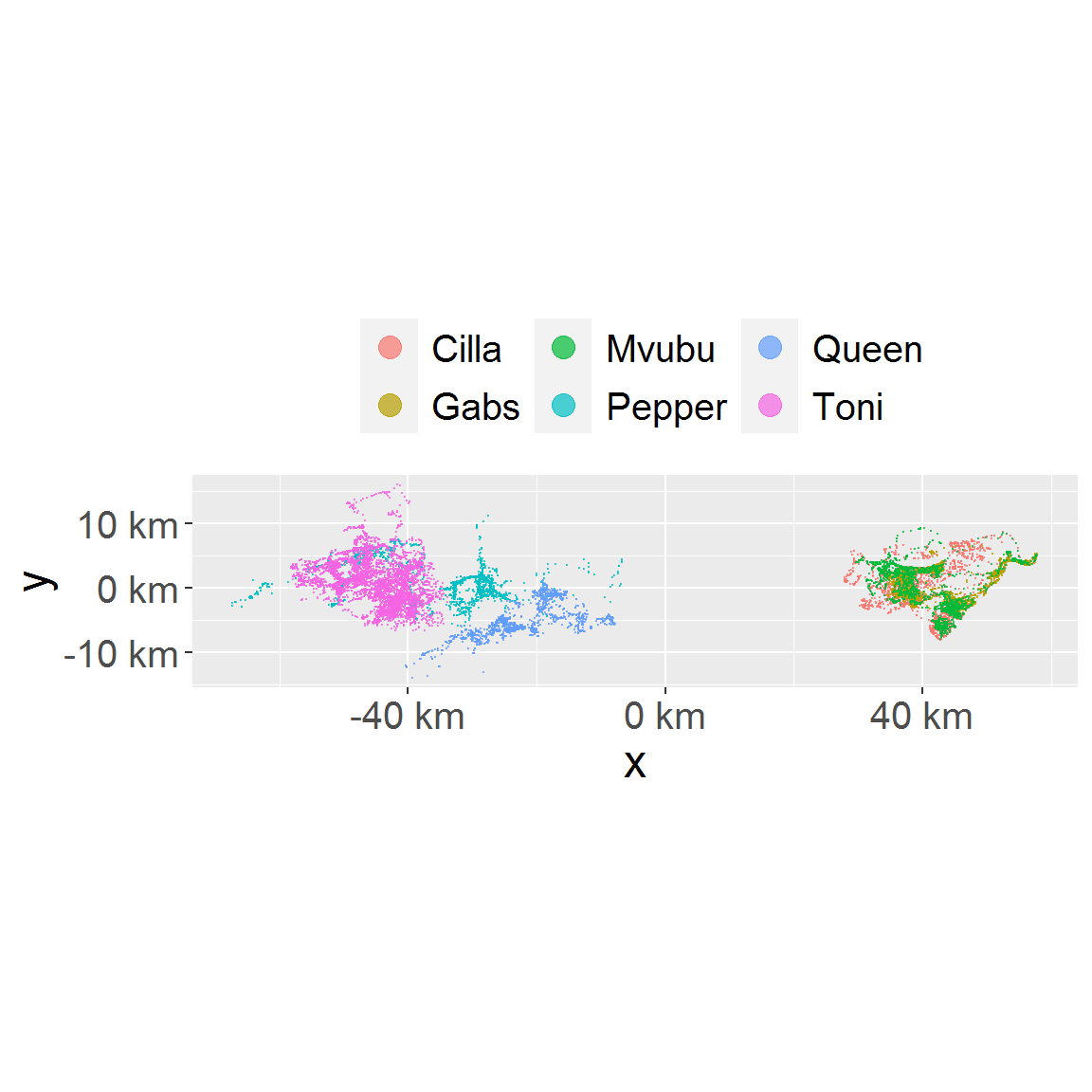
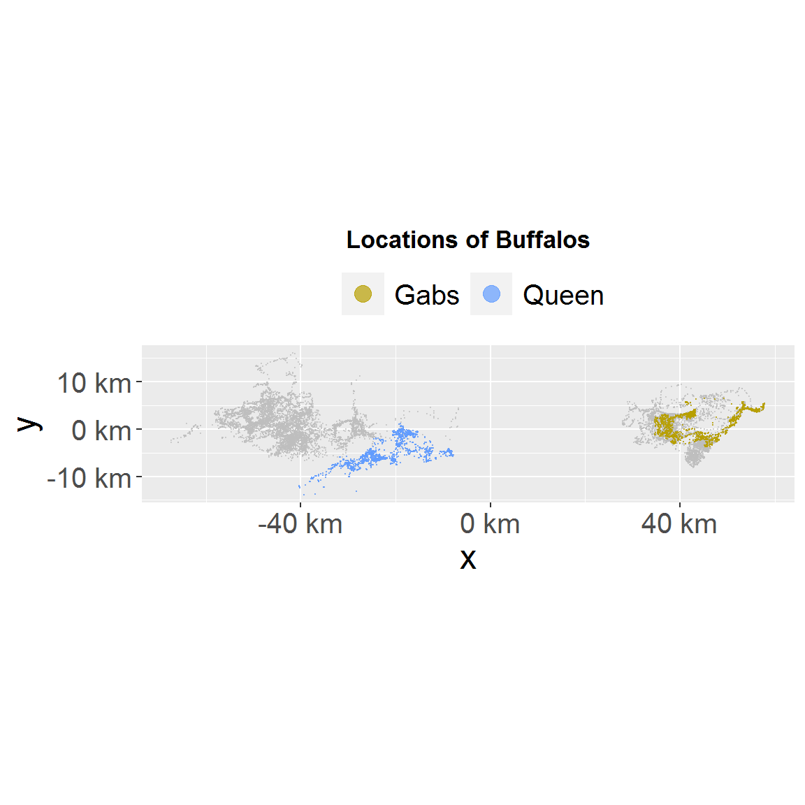
# plot animal locations
plot_loc(loc_data)
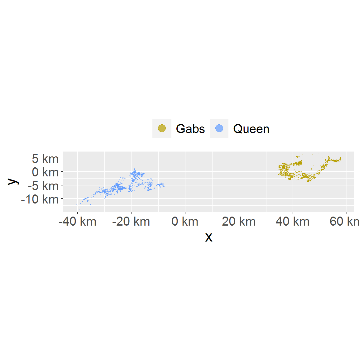
# plot a subset only. Note the color mapping is consistent because loc_data_sub1 id column hold all animal names in levels.
plot_loc(loc_data_sub1)
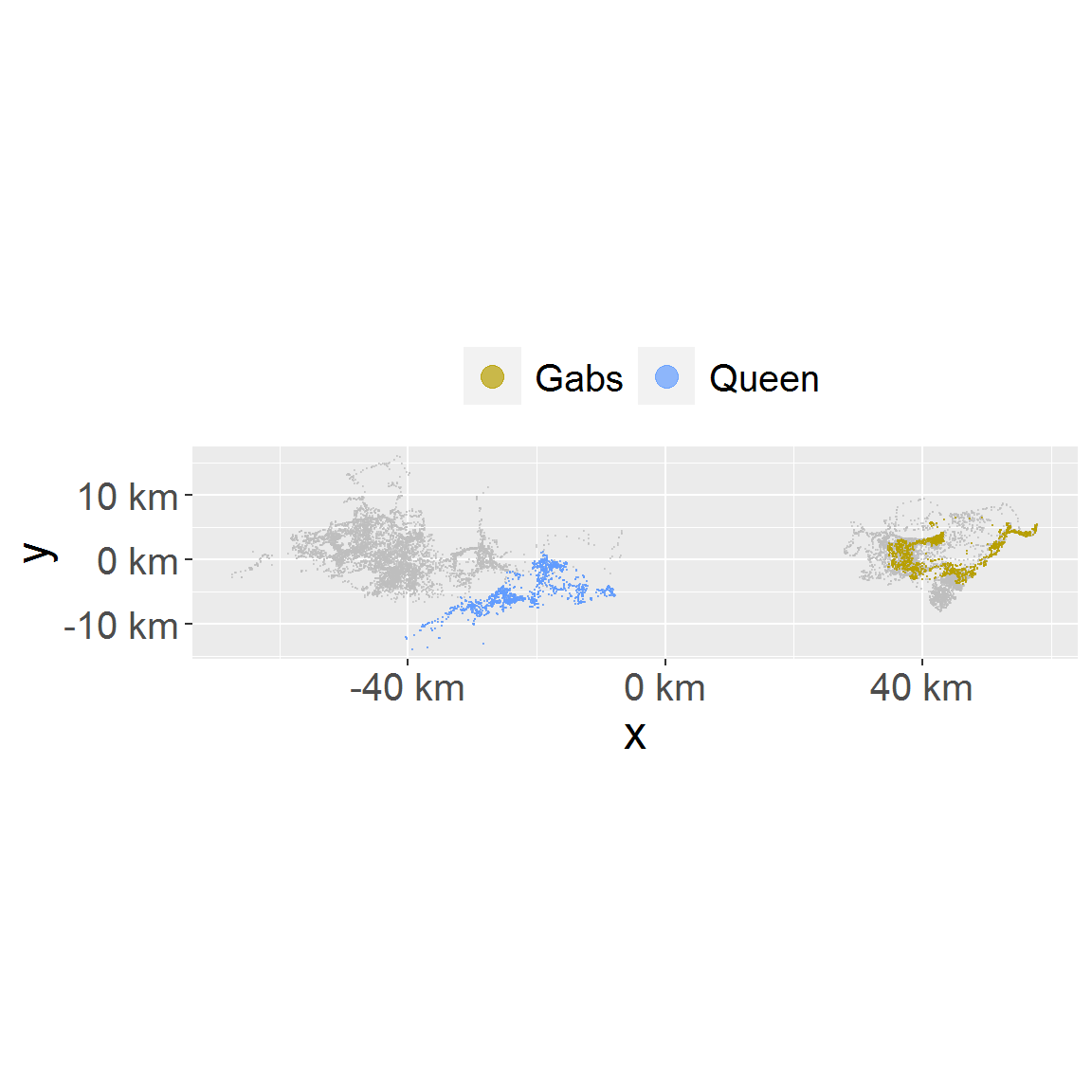
# with subset and full data set both provided, subset will be drawn with full data as background.
plot_loc(loc_data_sub1, loc_data)
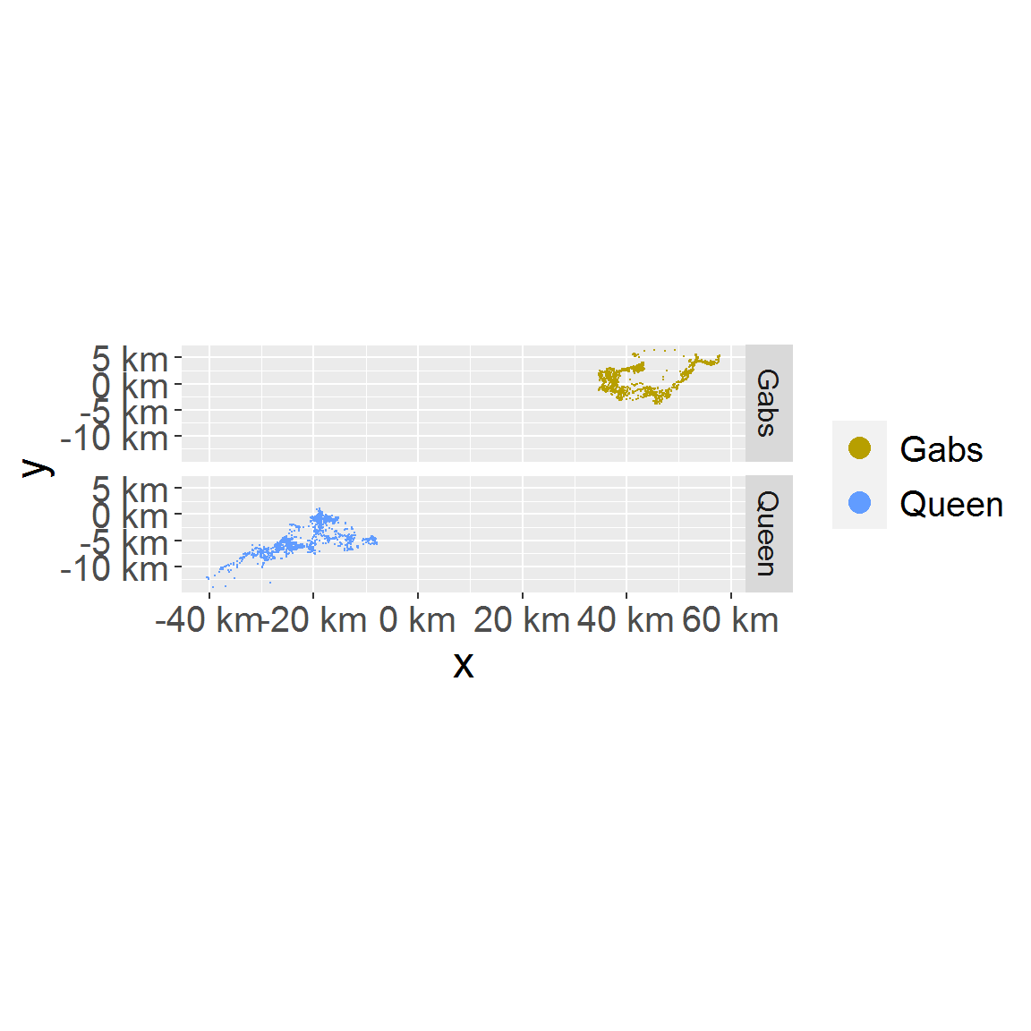
# location in facet
plot_loc_facet(loc_data_sub1)
# sampling time
plot_time(loc_data_sub1)

# take the ggplot2 object to further customize it
plot_loc(loc_data_sub1, loc_data) +
  ggplot2::ggtitle("Locations of Buffalos") +
  # override the default left alignment of title and make it bigger
  ctmmweb:::CENTER_TITLE
# export plot
g <- plot_loc(loc_data_sub1, loc_data)
# use this to save as file if needed
if (interactive()) {
  ggplot2::ggsave("test.png", g)
}
Variogram
We can plot both empirical variograms alone and empirical variograms with fitted theoretical semi-variance functions superimposed on them.
For example, to plot empirical variograms from telemetry data, one would do:
vario_list <- lapply(data_sample, ctmm::variogram)
# names of vario_list are needed for figure titles
names(vario_list) <- names(data_sample)
plot_vario(vario_list)

# sometimes the default figure settings doesn't work in some systems, you can clear the plot device then use a smaller title size
# dev.off()
# plot_vario(vario_list, cex = 0.55)
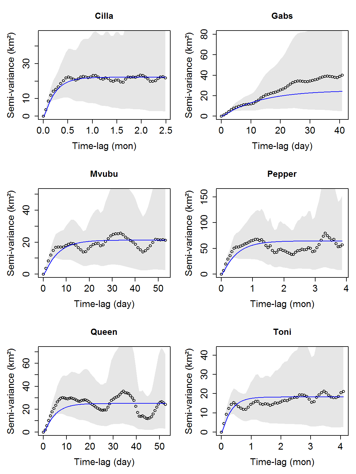
Similarly, we can compare initial movement model parameter guesses to the data via variograms:
guess_list <- lapply(data_sample,
                     function(tele)
                       ctmm::ctmm.guess(tele, interactive = FALSE))
plot_vario(vario_list, guess_list)
Model summary table
We can try different models on multiple animals in parallel.
Note there could be some known errors with data.table, R 3.4 and parallel operations. You can try to restart R session if met with same error.
# try multiple models in parallel with ctmm.select. parallel mode can be turned off with parallel = FALSE
model_try_res <- par_try_models(data_sample)
#> running parallel in SOCKET cluster of 6
# `model_try_res` holds a list of items named by animal names. Each item hold the attempted models for that animal as a sub list, named by model type.
print(str(model_try_res[1:3], max.level = 2))
#> List of 3
#>  $ Cilla:List of 6
#>   ..$ OU anisotropic :Formal class 'ctmm' [package "ctmm"]
#> @ info
#>   ..$ OUF anisotropic:Formal class 'ctmm' [package "ctmm"]
#> @ info
#>   ..$ OUf anisotropic:Formal class 'ctmm' [package "ctmm"]
#> @ info
#>   ..$ OU isotropic   :Formal class 'ctmm' [package "ctmm"]
#> @ info
#>   ..$ OUF isotropic  :Formal class 'ctmm' [package "ctmm"]
#> @ info
#>   ..$ IID anisotropic:Formal class 'ctmm' [package "ctmm"]
#> @ info
#>  $ Gabs :List of 6
#>   ..$ OU anisotropic :Formal class 'ctmm' [package "ctmm"]
#> @ info
#>   ..$ OUF anisotropic:Formal class 'ctmm' [package "ctmm"]
#> @ info
#>   ..$ OU isotropic   :Formal class 'ctmm' [package "ctmm"]
#> @ info
#>   ..$ OUF isotropic  :Formal class 'ctmm' [package "ctmm"]
#> @ info
#>   ..$ OUf anisotropic:Formal class 'ctmm' [package "ctmm"]
#> @ info
#>   ..$ IID anisotropic:Formal class 'ctmm' [package "ctmm"]
#> @ info
#>  $ Mvubu:List of 6
#>   ..$ OU anisotropic :Formal class 'ctmm' [package "ctmm"]
#> @ info
#>   ..$ OUF anisotropic:Formal class 'ctmm' [package "ctmm"]
#> @ info
#>   ..$ OUf anisotropic:Formal class 'ctmm' [package "ctmm"]
#> @ info
#>   ..$ OU isotropic   :Formal class 'ctmm' [package "ctmm"]
#> @ info
#>   ..$ OUF isotropic  :Formal class 'ctmm' [package "ctmm"]
#> @ info
#>   ..$ IID anisotropic:Formal class 'ctmm' [package "ctmm"]
#> @ info
#> NULL
# a data.table of models information summary
model_summary <- summary_tried_models(model_try_res)
# you can also open it with RStudio's data.frame viewer
knitr::kable(model_summary)
| model_no | identity | model_type | model_name | ΔAICc | DOF mean | DOF area | DOF speed | area (km²) | area CI (km²) | τ[position] (days) | τ[position] CI (days) | τ[velocity] (hours) | τ[velocity] CI (hours) | speed (km/day) | speed CI (km/day) | τ | τ[decay] | τ[period] |
|---|---|---|---|---|---|---|---|---|---|---|---|---|---|---|---|---|---|---|
| 1 | Cilla | OU anisotropic | 1. Cilla - OU anisotropic | 0.00 | 15.35 | 26.43 | 0.00 | 403.54 | (264.63 - 571.29) | 5.07 | (2.85 - 9.04) | NA | NA | NA | NA | NA | NA | NA |
| 2 | Cilla | OUF anisotropic | 2. Cilla - OUF anisotropic | 2.23 | 15.43 | 26.68 | 0.00 | 402.78 | (264.71 - 569.37) | 5.04 | (2.1 - 12.07) | 0.16 | (0 - 13.44) | 38.88 | (0 - 358.56) | NA | NA | NA |
| 3 | Cilla | OUf anisotropic | 3. Cilla - OUf anisotropic | 13.28 | 30.37 | 50.23 | 62.26 | 363.74 | (270.17 - 471.01) | NA | NA | NA | NA | 5.18 | (4.32 - 6.05) | 107343.94 | NA | NA |
| 4 | Cilla | OU isotropic | 4. Cilla - OU isotropic | 24.57 | 16.89 | 29.29 | 0.00 | 432.94 | (290.58 - 603.23) | 4.58 | (2.64 - 7.93) | NA | NA | NA | NA | NA | NA | NA |
| 5 | Cilla | OUF isotropic | 5. Cilla - OUF isotropic | 26.52 | 17.74 | 30.59 | 0.15 | 431.56 | (292.39 - 597.38) | 4.25 | (1.77 - 10.24) | 2.34 | (0 - 15.21) | 10.37 | (0 - 31.1) | NA | NA | NA |
| 6 | Cilla | IID anisotropic | 6. Cilla - IID anisotropic | 150.13 | 100.00 | 98.69 | 0.00 | 385.39 | (313.12 - 465.05) | NA | NA | NA | NA | NA | NA | NA | NA | NA |
| 7 | Gabs | OU anisotropic | 7. Gabs - OU anisotropic | 0.00 | 4.79 | 6.55 | 0.00 | 409.20 | (158.33 - 777.09) | 10.93 | (2.22 - 53.84) | NA | NA | NA | NA | NA | NA | NA |
| 8 | Gabs | OUF anisotropic | 8. Gabs - OUF anisotropic | 2.00 | 5.53 | 11.40 | 0.00 | 347.40 | (175.93 - 576.23) | 9.14 | (3.61 - 23.16) | 0.00 | (0 - 0.13) | NA | NA | NA | NA | NA |
| 9 | Gabs | OU isotropic | 9. Gabs - OU isotropic | 15.42 | 3.93 | 5.30 | 0.00 | 574.22 | (194.12 - 1156.77) | 14.17 | (1.74 - 115.47) | NA | NA | NA | NA | NA | NA | NA |
| 10 | Gabs | OUF isotropic | 10. Gabs - OUF isotropic | 17.31 | 4.58 | 9.89 | 0.00 | 475.35 | (226.87 - 814.17) | 11.57 | (4.14 - 32.38) | 0.00 | (0 - 0.35) | NA | NA | NA | NA | NA |
| 11 | Gabs | OUf anisotropic | 11. Gabs - OUf anisotropic | 51.09 | 19.79 | 32.65 | 71.32 | 278.53 | (191.31 - 381.87) | NA | NA | NA | NA | 5.18 | (4.32 - 6.05) | 94919.23 | NA | NA |
| 12 | Gabs | IID anisotropic | 12. Gabs - IID anisotropic | 306.86 | 100.00 | 120.27 | 0.00 | 277.28 | (229.94 - 328.98) | NA | NA | NA | NA | NA | NA | NA | NA | NA |
| 13 | Mvubu | OU anisotropic | 13. Mvubu - OU anisotropic | 0.00 | 12.62 | 20.08 | 0.00 | 398.19 | (243.51 - 590.28) | 4.56 | (2.31 - 9.03) | NA | NA | NA | NA | NA | NA | NA |
| 14 | Mvubu | OUF anisotropic | 14. Mvubu - OUF anisotropic | 0.57 | 14.62 | 22.98 | 3.23 | 394.75 | (250.17 - 571.77) | 3.71 | (1.57 - 8.78) | 4.52 | (0 - 10.94) | 8.64 | (4.32 - 12.96) | NA | NA | NA |
| 15 | Mvubu | OUf anisotropic | 15. Mvubu - OUf anisotropic | 8.20 | 26.93 | 42.48 | 66.93 | 349.79 | (252.61 - 462.55) | NA | NA | NA | NA | 6.91 | (6.05 - 6.91) | 88381.02 | NA | NA |
| 16 | Mvubu | OU isotropic | 16. Mvubu - OU isotropic | 26.35 | 14.30 | 24.00 | 0.00 | 418.53 | (268.15 - 601.83) | 3.98 | (2.16 - 7.34) | NA | NA | NA | NA | NA | NA | NA |
| 17 | Mvubu | OUF isotropic | 17. Mvubu - OUF isotropic | 27.77 | 15.70 | 26.19 | 0.91 | 415.21 | (271.68 - 588.69) | 3.48 | (1.53 - 7.95) | 2.97 | (0 - 10.03) | 10.37 | (1.73 - 19.87) | NA | NA | NA |
| 18 | Mvubu | IID anisotropic | 18. Mvubu - IID anisotropic | 167.71 | 100.00 | 99.24 | 0.00 | 353.33 | (287.25 - 426.16) | NA | NA | NA | NA | NA | NA | NA | NA | NA |
| 19 | Pepper | OUF anisotropic | 19. Pepper - OUF anisotropic | 0.00 | 17.81 | 25.69 | 30.66 | 681.98 | (444.21 - 969.89) | 6.62 | (3.2 - 13.69) | 12.05 | (6.13 - 23.72) | 5.18 | (4.32 - 6.05) | NA | NA | NA |
| 20 | Pepper | OUf anisotropic | 20. Pepper - OUf anisotropic | 11.03 | 33.35 | 47.33 | 45.09 | 587.49 | (432.17 - 766.29) | NA | NA | NA | NA | 5.18 | (4.32 - 6.05) | 151019.36 | NA | NA |
| 21 | Pepper | OU anisotropic | 21. Pepper - OU anisotropic | 14.03 | 13.13 | 19.42 | 0.00 | 690.12 | (418.06 - 1029.25) | 10.01 | (4.97 - 20.18) | NA | NA | NA | NA | NA | NA | NA |
| 22 | Pepper | OUF isotropic | 22. Pepper - OUF isotropic | 43.40 | 13.43 | 20.88 | 44.82 | 1153.83 | (713.15 - 1698.83) | 9.28 | (4.36 - 19.74) | 12.72 | (7.02 - 23.05) | 5.18 | (4.32 - 6.05) | NA | NA | NA |
| 23 | Queen | OU anisotropic | 23. Queen - OU anisotropic | 0.00 | 10.17 | 15.75 | 0.00 | 293.45 | (166.89 - 455.13) | 4.92 | (2.27 - 10.67) | NA | NA | NA | NA | NA | NA | NA |
| 24 | Queen | OUF anisotropic | 24. Queen - OUF anisotropic | 0.29 | 11.25 | 17.12 | 3.32 | 298.54 | (174.28 - 455.71) | 4.23 | (1.85 - 9.66) | 2.86 | (0 - 6.51) | 8.64 | (4.32 - 13.82) | NA | NA | NA |
| 25 | Queen | OUf anisotropic | 25. Queen - OUf anisotropic | 20.76 | 24.50 | 36.04 | 58.55 | 266.01 | (186.35 - 359.63) | NA | NA | NA | NA | 6.91 | (6.05 - 7.78) | 76354.22 | NA | NA |
| 26 | Queen | OUF isotropic | 26. Queen - OUF isotropic | 33.98 | 10.60 | 16.38 | 31.13 | 469.21 | (270.21 - 722.22) | 4.43 | (1.81 - 10.82) | 6.12 | (2.54 - 14.73) | 6.91 | (5.18 - 7.78) | NA | NA | NA |
| 27 | Queen | OU isotropic | 27. Queen - OU isotropic | 42.41 | 8.12 | 12.51 | 0.00 | 471.97 | (247.76 - 767.22) | 6.55 | (2.68 - 16.01) | NA | NA | NA | NA | NA | NA | NA |
| 28 | Queen | IID anisotropic | 28. Queen - IID anisotropic | 226.94 | 100.00 | 70.40 | 0.00 | 254.93 | (198.88 - 317.83) | NA | NA | NA | NA | NA | NA | NA | NA | NA |
| 29 | Toni | OUf anisotropic | 29. Toni - OUf anisotropic | 0.00 | 34.36 | 51.63 | 53.37 | 322.98 | (240.95 - 416.85) | NA | NA | NA | NA | 3.46 | (2.59 - 3.46) | 156130.99 | NA | NA |
| 30 | Toni | OU anisotropic | 30. Toni - OU anisotropic | 0.05 | 21.80 | 35.35 | 0.00 | 341.21 | (238.14 - 462.54) | 5.75 | (3.38 - 9.77) | NA | NA | NA | NA | NA | NA | NA |
| 31 | Toni | OUF anisotropic | 31. Toni - OUF anisotropic | 0.37 | 25.88 | 39.80 | 4.85 | 337.96 | (241.22 - 450.75) | 4.27 | (1.56 - 11.69) | 13.79 | (0 - 32.43) | 3.46 | (2.59 - 5.18) | NA | NA | NA |
| 32 | Toni | OUF isotropic | 32. Toni - OUF isotropic | 0.44 | 23.77 | 38.78 | 2.59 | 358.13 | (254.39 - 479.33) | 4.83 | (1.95 - 11.94) | 11.18 | (0 - 29.59) | 4.32 | (1.73 - 6.91) | NA | NA | NA |
| 33 | Toni | OUf isotropic | 33. Toni - OUf isotropic | 1.51 | 33.49 | 52.31 | 60.73 | 342.06 | (255.7 - 440.78) | NA | NA | NA | NA | 3.46 | (2.59 - 3.46) | 160366.84 | NA | NA |
| 34 | Toni | OUΩ anisotropic | 34. Toni - OUΩ anisotropic | 2.24 | 34.36 | 51.63 | 53.37 | 322.98 | (240.95 - 416.85) | NA | NA | NA | NA | 3.46 | (2.59 - 3.46) | NA | 156131 | 98338578462 |
| 35 | Toni | IID anisotropic | 35. Toni - IID anisotropic | 88.06 | 100.00 | 97.61 | 0.00 | 309.00 | (250.75 - 373.24) | NA | NA | NA | NA | NA | NA | NA | NA | NA |
There could be multiple models attempted for each animal. In the webapp you can select a subset of models then check their variograms, home ranges and occurrences. You can also select a subset of fitted models via in a script as:
To make selecting a subset easier, we first convert this nested list structure to a flat list:
# the nested structure of model fit result
names(model_try_res)
#> [1] "Cilla"  "Gabs"   "Mvubu"  "Pepper" "Queen"  "Toni"
names(model_try_res[[1]])
#> [1] "OU anisotropic"  "OUF anisotropic" "OUf anisotropic" "OU isotropic"
#> [5] "OUF isotropic"   "IID anisotropic"
# convert to a flat list
model_list <- flatten_models(model_try_res)
names(model_list)
#>  [1] "1. Cilla - OU anisotropic"    "2. Cilla - OUF anisotropic"
#>  [3] "3. Cilla - OUf anisotropic"   "4. Cilla - OU isotropic"
#>  [5] "5. Cilla - OUF isotropic"     "6. Cilla - IID anisotropic"
#>  [7] "7. Gabs - OU anisotropic"     "8. Gabs - OUF anisotropic"
#>  [9] "9. Gabs - OU isotropic"       "10. Gabs - OUF isotropic"
#> [11] "11. Gabs - OUf anisotropic"   "12. Gabs - IID anisotropic"
#> [13] "13. Mvubu - OU anisotropic"   "14. Mvubu - OUF anisotropic"
#> [15] "15. Mvubu - OUf anisotropic"  "16. Mvubu - OU isotropic"
#> [17] "17. Mvubu - OUF isotropic"    "18. Mvubu - IID anisotropic"
#> [19] "19. Pepper - OUF anisotropic" "20. Pepper - OUf anisotropic"
#> [21] "21. Pepper - OU anisotropic"  "22. Pepper - OUF isotropic"
#> [23] "23. Queen - OU anisotropic"   "24. Queen - OUF anisotropic"
#> [25] "25. Queen - OUf anisotropic"  "26. Queen - OUF isotropic"
#> [27] "27. Queen - OU isotropic"     "28. Queen - IID anisotropic"
#> [29] "29. Toni - OUf anisotropic"   "30. Toni - OU anisotropic"
#> [31] "31. Toni - OUF anisotropic"   "32. Toni - OUF isotropic"
#> [33] "33. Toni - OUf isotropic"     "34. Toni - OU惟 anisotropic"
#> [35] "35. Toni - IID anisotropic"
Then we can find the model names in the model summary table by model_no or model_type. The code here uses data.table syntax, but you can also use the table as data.frame if you want.
# select subset in model summary table by model_no
knitr::kable(model_summary[model_no %in% c(1, 3, 10, 11, 12, 13)])
| model_no | identity | model_type | model_name | ΔAICc | DOF mean | DOF area | DOF speed | area (km²) | area CI (km²) | τ[position] (days) | τ[position] CI (days) | τ[velocity] (hours) | τ[velocity] CI (hours) | speed (km/day) | speed CI (km/day) | τ | τ[decay] | τ[period] |
|---|---|---|---|---|---|---|---|---|---|---|---|---|---|---|---|---|---|---|
| 1 | Cilla | OU anisotropic | 1. Cilla - OU anisotropic | 0.00 | 15.35 | 26.43 | 0.00 | 403.54 | (264.63 - 571.29) | 5.07 | (2.85 - 9.04) | NA | NA | NA | NA | NA | NA | NA |
| 3 | Cilla | OUf anisotropic | 3. Cilla - OUf anisotropic | 13.28 | 30.37 | 50.23 | 62.26 | 363.74 | (270.17 - 471.01) | NA | NA | NA | NA | 5.18 | (4.32 - 6.05) | 107343.94 | NA | NA |
| 10 | Gabs | OUF isotropic | 10. Gabs - OUF isotropic | 17.31 | 4.58 | 9.89 | 0.00 | 475.35 | (226.87 - 814.17) | 11.57 | (4.14 - 32.38) | 0 | (0 - 0.35) | NA | NA | NA | NA | NA |
| 11 | Gabs | OUf anisotropic | 11. Gabs - OUf anisotropic | 51.09 | 19.79 | 32.65 | 71.32 | 278.53 | (191.31 - 381.87) | NA | NA | NA | NA | 5.18 | (4.32 - 6.05) | 94919.23 | NA | NA |
| 12 | Gabs | IID anisotropic | 12. Gabs - IID anisotropic | 306.86 | 100.00 | 120.27 | 0.00 | 277.28 | (229.94 - 328.98) | NA | NA | NA | NA | NA | NA | NA | NA | NA |
| 13 | Mvubu | OU anisotropic | 13. Mvubu - OU anisotropic | 0.00 | 12.62 | 20.08 | 0.00 | 398.19 | (243.51 - 590.28) | 4.56 | (2.31 - 9.03) | NA | NA | NA | NA | NA | NA | NA |
# select by model type
knitr::kable(model_summary[model_type == "OU anisotropic"])
| model_no | identity | model_type | model_name | ΔAICc | DOF mean | DOF area | DOF speed | area (km²) | area CI (km²) | τ[position] (days) | τ[position] CI (days) | τ[velocity] (hours) | τ[velocity] CI (hours) | speed (km/day) | speed CI (km/day) | τ | τ[decay] | τ[period] |
|---|---|---|---|---|---|---|---|---|---|---|---|---|---|---|---|---|---|---|
| 1 | Cilla | OU anisotropic | 1. Cilla - OU anisotropic | 0.00 | 15.35 | 26.43 | 0 | 403.54 | (264.63 - 571.29) | 5.07 | (2.85 - 9.04) | NA | NA | NA | NA | NA | NA | NA |
| 7 | Gabs | OU anisotropic | 7. Gabs - OU anisotropic | 0.00 | 4.79 | 6.55 | 0 | 409.20 | (158.33 - 777.09) | 10.93 | (2.22 - 53.84) | NA | NA | NA | NA | NA | NA | NA |
| 13 | Mvubu | OU anisotropic | 13. Mvubu - OU anisotropic | 0.00 | 12.62 | 20.08 | 0 | 398.19 | (243.51 - 590.28) | 4.56 | (2.31 - 9.03) | NA | NA | NA | NA | NA | NA | NA |
| 21 | Pepper | OU anisotropic | 21. Pepper - OU anisotropic | 14.03 | 13.13 | 19.42 | 0 | 690.12 | (418.06 - 1029.25) | 10.01 | (4.97 - 20.18) | NA | NA | NA | NA | NA | NA | NA |
| 23 | Queen | OU anisotropic | 23. Queen - OU anisotropic | 0.00 | 10.17 | 15.75 | 0 | 293.45 | (166.89 - 455.13) | 4.92 | (2.27 - 10.67) | NA | NA | NA | NA | NA | NA | NA |
| 30 | Toni | OU anisotropic | 30. Toni - OU anisotropic | 0.05 | 21.80 | 35.35 | 0 | 341.21 | (238.14 - 462.54) | 5.75 | (3.38 - 9.77) | NA | NA | NA | NA | NA | NA | NA |
# select first(best) model for each animal using the smallest AICc value
knitr::kable(model_summary[`ΔAICc` == 0])
| model_no | identity | model_type | model_name | ΔAICc | DOF mean | DOF area | DOF speed | area (km²) | area CI (km²) | τ[position] (days) | τ[position] CI (days) | τ[velocity] (hours) | τ[velocity] CI (hours) | speed (km/day) | speed CI (km/day) | τ | τ[decay] | τ[period] |
|---|---|---|---|---|---|---|---|---|---|---|---|---|---|---|---|---|---|---|
| 1 | Cilla | OU anisotropic | 1. Cilla - OU anisotropic | 0 | 15.35 | 26.43 | 0.00 | 403.54 | (264.63 - 571.29) | 5.07 | (2.85 - 9.04) | NA | NA | NA | NA | NA | NA | NA |
| 7 | Gabs | OU anisotropic | 7. Gabs - OU anisotropic | 0 | 4.79 | 6.55 | 0.00 | 409.20 | (158.33 - 777.09) | 10.93 | (2.22 - 53.84) | NA | NA | NA | NA | NA | NA | NA |
| 13 | Mvubu | OU anisotropic | 13. Mvubu - OU anisotropic | 0 | 12.62 | 20.08 | 0.00 | 398.19 | (243.51 - 590.28) | 4.56 | (2.31 - 9.03) | NA | NA | NA | NA | NA | NA | NA |
| 19 | Pepper | OUF anisotropic | 19. Pepper - OUF anisotropic | 0 | 17.81 | 25.69 | 30.66 | 681.98 | (444.21 - 969.89) | 6.62 | (3.2 - 13.69) | 12.05 | (6.13 - 23.72) | 5.18 | (4.32 - 6.05) | NA | NA | NA |
| 23 | Queen | OU anisotropic | 23. Queen - OU anisotropic | 0 | 10.17 | 15.75 | 0.00 | 293.45 | (166.89 - 455.13) | 4.92 | (2.27 - 10.67) | NA | NA | NA | NA | NA | NA | NA |
| 29 | Toni | OUf anisotropic | 29. Toni - OUf anisotropic | 0 | 34.36 | 51.63 | 53.37 | 322.98 | (240.95 - 416.85) | NA | NA | NA | NA | 3.46 | (2.59 - 3.46) | 156131 | NA | NA |
# The expression is enclosed with () to enable automatical printing of result. Both model_name and identity are selected in same filter. We need the model_name to filter the model list, and the animal name to filter the variograms
(names_sub2 <- model_summary[(model_no %in% c(1, 3, 10, 11, 12, 13)),
                             .(model_name, identity)])
#>                    model_name identity
#> 1:  1. Cilla - OU anisotropic    Cilla
#> 2: 3. Cilla - OUf anisotropic    Cilla
#> 3:   10. Gabs - OUF isotropic     Gabs
#> 4: 11. Gabs - OUf anisotropic     Gabs
#> 5: 12. Gabs - IID anisotropic     Gabs
#> 6: 13. Mvubu - OU anisotropic    Mvubu
Once you have selected the models in summary table, you can filter the actual models list with model names. Note this is a different subset from loc_data_sub1 above.
# filter model list by model names to get subset of model list.
model_list_sub2 <- model_list[names_sub2$model_name]
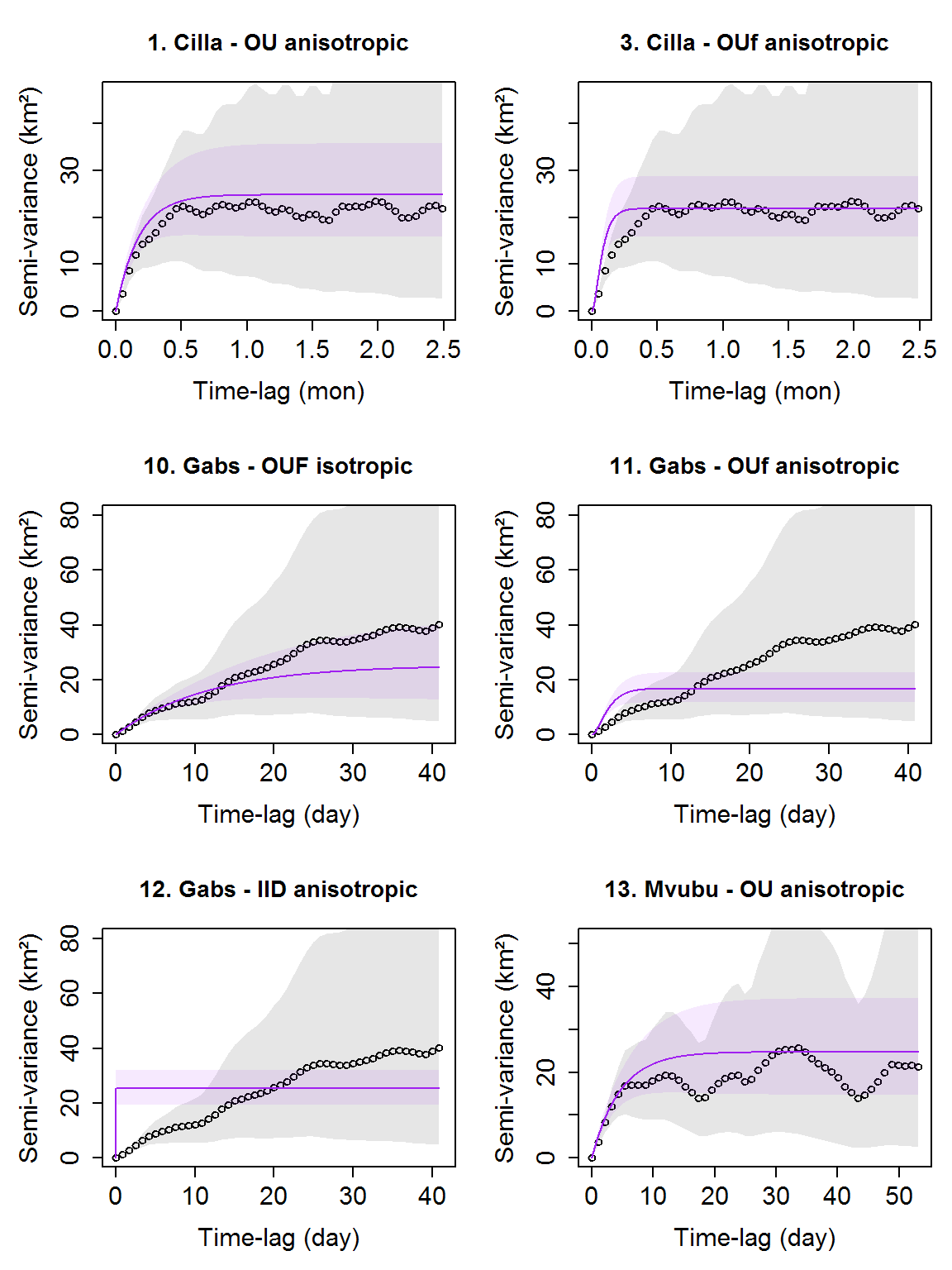
Now we can plot variograms with the fitted SVFs of the selected models. Note the vario_list_sub2 needs to match with model_list_sub2 in length and animal name, so they are based on same data.
# get corresponding variograms by animal names.
vario_list_sub2 <- vario_list[names_sub2$identity]
# specify a different color for model
plot_vario(vario_list_sub2, model_list_sub2, model_color = "purple")
Home range
We can estimate home range with the telemetry data and the fitted models. Note parallel mode is not used because we want to calculate all animals together to put them in same grid.
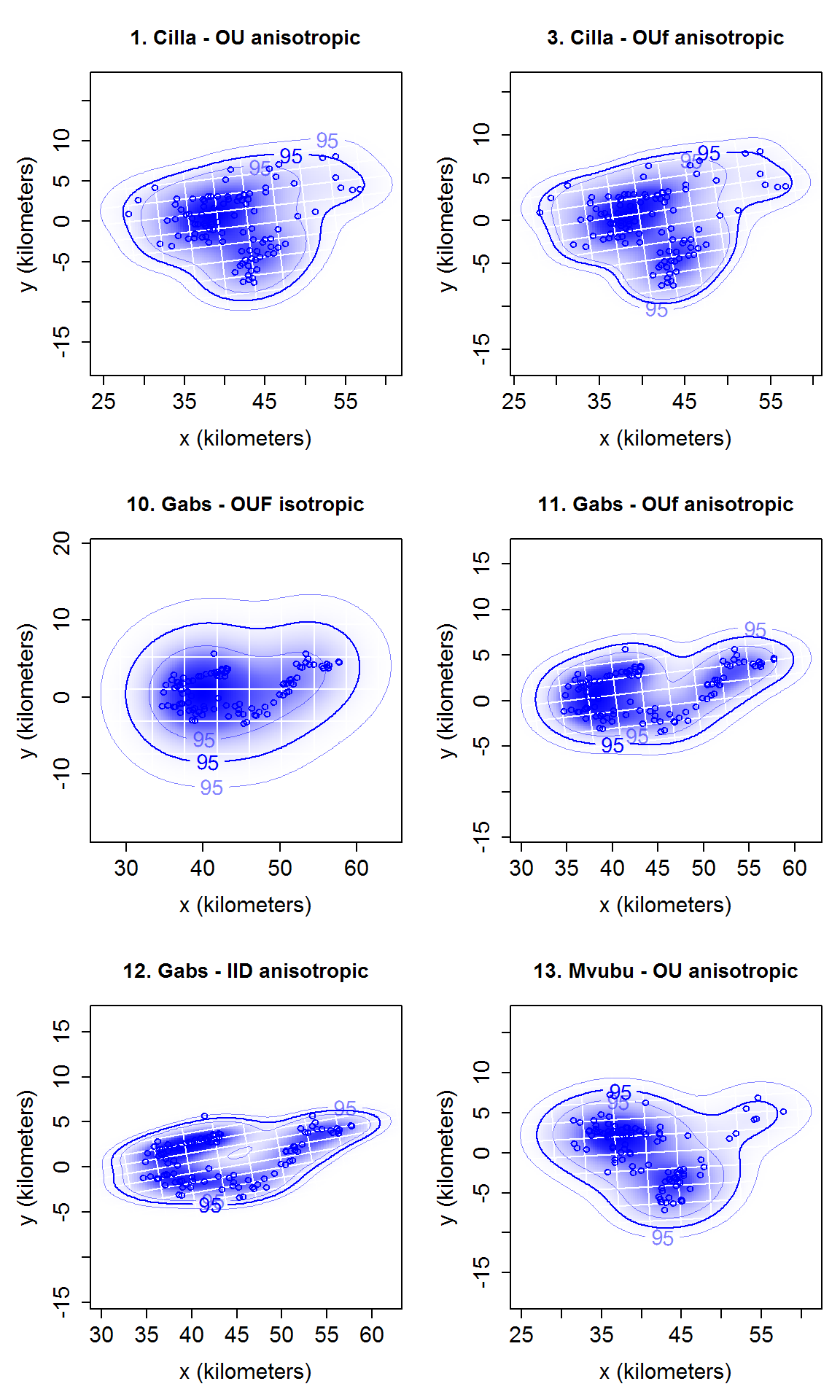
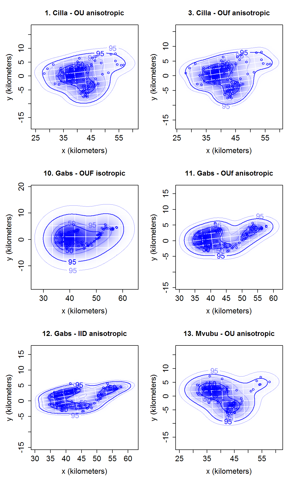
# calculate home range with ctmm::akde.
tele_list_sub2 <- data_sample[names_sub2$identity]
hrange_list_sub2 <- akde(tele_list_sub2, CTMM = model_list_sub2)
# name by model name
names(hrange_list_sub2) <- names(model_list_sub2)
# summary of each home range. There is no summary table function here because we borrowed the model table in app to make the home range summay table. To reproduce that in functions need model table/model_try_res and the selection as parameters, which will be quite awkward. If there is a strong request from users, a summary table function can be added.
lapply(hrange_list_sub2, summary)
#> $`1. Cilla - OU anisotropic`
#> $`1. Cilla - OU anisotropic`$DOF
#>      area bandwidth
#>  26.43320  42.92138
#>
#> $`1. Cilla - OU anisotropic`$CI
#>                               low      est     high
#> area (square kilometers) 238.1235 363.1199 514.0671
#>
#>
#> $`3. Cilla - OUf anisotropic`
#> $`3. Cilla - OUf anisotropic`$DOF
#>      area bandwidth
#>  50.22548  67.22177
#>
#> $`3. Cilla - OUf anisotropic`$CI
#>                               low      est     high
#> area (square kilometers) 248.4837 334.5437 433.2031
#>
#>
#> $`10. Gabs - OUF isotropic`
#> $`10. Gabs - OUF isotropic`$DOF
#>      area bandwidth
#>  9.891746  8.309818
#>
#> $`10. Gabs - OUF isotropic`$CI
#>                               low      est     high
#> area (square kilometers) 209.8107 439.6118 752.9657
#>
#>
#> $`11. Gabs - OUf anisotropic`
#> $`11. Gabs - OUf anisotropic`$DOF
#>      area bandwidth
#>  32.65113  40.72327
#>
#> $`11. Gabs - OUf anisotropic`$CI
#>                              low      est     high
#> area (square kilometers) 161.681 235.3929 322.7311
#>
#>
#> $`12. Gabs - IID anisotropic`
#> $`12. Gabs - IID anisotropic`$DOF
#>      area bandwidth
#> 120.27079  99.99999
#>
#> $`12. Gabs - IID anisotropic`$CI
#>                              low      est     high
#> area (square kilometers) 172.078 207.5022 246.1927
#>
#>
#> $`13. Mvubu - OU anisotropic`
#> $`13. Mvubu - OU anisotropic`$DOF
#>      area bandwidth
#>  20.08493  32.98463
#>
#> $`13. Mvubu - OU anisotropic`$CI
#>                               low      est     high
#> area (square kilometers) 206.9929 338.4765 501.7671
# plot home range
plot_ud(hrange_list_sub2)

# plot home range with location overlay
plot_ud(hrange_list_sub2, tele_list = tele_list_sub2)
# plot with different level.UD values
plot_ud(hrange_list_sub2, level_vec = c(0.50, 0.95), tele_list = tele_list_sub2)
Batch script for home range
Home range is one of the most used feature in ctmm/ctmmweb. Sometimes you have lots of individuals and don’t need to fine tune each model, then you can calculate home range in batch mode. ctmmweb package provided many functions to make this process as easy as possible. Check the function documents for more details.
The script can also be used to create a reproducible example if you met any error in modeling/home range parts.
library(ctmm)
library(ctmmweb)
library(data.table)

# this read from a .rds from saved progress file. You can also import your data directly with as.telemetry
tele_list <- readRDS("/Users/xhdong/Downloads/Saved_2019-11-15_11-37-41_models/input_telemetry.rds")
# one line to try models. The result is a nested list of CTMM models
model_try_res <- par_try_models(tele_list)
save.image("test.RData")
# summary models to find the best
model_summary <- summary_tried_models(model_try_res)
# select the best model name for each individual, which is the first one with 0 AICc
best_model_names <- model_summary[, .(best_model_name = model_name[1]),
                                  by = "identity"]$best_model_name
# get a flat list of model object
model_list <- flatten_models(model_try_res)
# get the best model objects
best_models <- model_list[best_model_names]
# calculate home range in same grid, with optimal weighting on
hrange_list_same_grid <- akde(tele_list, best_models,
                              weights = TRUE)
# calculate home range separately, with optimal weighting on
hrange_list <- par_hrange_each(tele_list, best_models,
                               rep.int(list(TRUE), length(tele_list)))
Occurrence
Occurrence distribution can be calculated from the telemetry data and the fitted models in parallel.
# calculate occurrence in parallel. parallel can be disabled with fallback = TRUE
occur_list_sub2 <- par_occur(tele_list_sub2, model_list_sub2)
#> running parallel in SOCKET cluster of 6
# plot occurrence. Note tele_list is not needed here because the location overlay usually interfere with occurrence plot.
plot_ud(occur_list_sub2, level_vec = c(0.50, 0.95))

Maps
We can then build interactive online maps of the data and fitted Home Range and Occurrence distributions. For example, one can display the location data on a map via:
# loc_data_sub1 is used for visualization plot. all the model selections above are based on a different subset. We need to get corresponding loc_data subset for model selections
loc_data_sub2 <- loc_data[identity %in% names(tele_list_sub2)]
point_map(loc_data_sub2)
point_map(loc_data)
The map can be saved as a self contained html file.
# save map to single html file. file can only be a filename, not a relative path
if(interactive()) {
  htmlwidgets::saveWidget(point_map(loc_data_sub2), file = "point_map.html")
}
Displaying home range estimates requires more input. See their help documents for detailed explanations.
# A map with home range estimates need: list of home range UD object, vector of level.UD in ctmm::plot.telemetry, a vector of color names for each home range estimate.
range_map(hrange_list_sub2, 0.95, rainbow(length(hrange_list_sub2)))
# To overlay home range estimates with animal locations, the corresponding animal location data is needed.
point_range_map(loc_data_sub2, hrange_list_sub2, 0.95,
                rainbow(length(hrange_list_sub2)))